LAPLACE TRANSFORM AS AN USEFUL TOOL IN TRANSIENT


 to")

,")

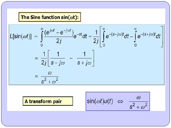


 formula is a general case of Fourier integral")


 If the denominator has also the solution s=0, then the Laplace image F(s")


, the equivalent operational circuit is given in the Fig. 1")


- Slides: 69
LAPLACE TRANSFORM AS AN USEFUL TOOL IN TRANSIENT STATE ANALYSIS Oana Mihaela Drosu Dr. Eng. , Lecturer POLITEHNICA University of Bucharest Department of Electrical Engineering LPP Erasmus+
PART I INTRODUCTION TO LAPLACE TRANSFORM THEORY
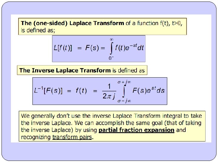
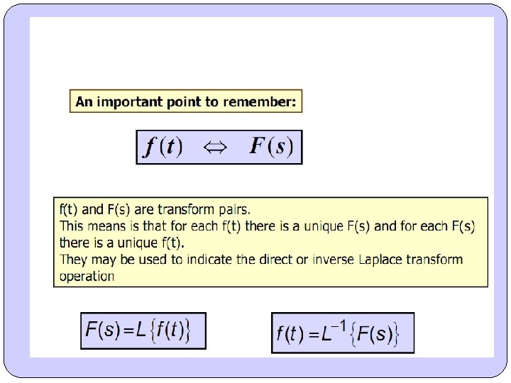
Definition The Laplace transform is a linear operator that switched a function f(t) to F(s), where s = s+wj. (Go from time argument with real input to a complex angular frequency input). Note that the real part s of the complex variable s must be large enough for the integral to converge.
Restrictions There are two governing factors that determine whether Laplace transforms can be used: • f(t) must be at least piecewise continuous for t ≥ 0 • |f(t)| ≤ Meγt where M and γ are constants
Conditions • to be limited and integrable on any interval (t 1, t 2), where 0< t 1< t 2 ; • to be absolute integrable on the interval [0, t 0 ], where t 0 >0; • at least one value s=s 0, to exist for the integral to have sense; • if it is absolute convergent for s=s 0, then it will be generally absolute convergent :
• In these conditions we can find a minimum value of Re{s}, denoted , for the Laplace transform of f(t) to exist (this is simple convergence abscissa); • The definition domain for F(s) is the complex semiplane at the right of :
BIBLIOGRAPHY: • Norman Balabanian: Electric Circuits; Mc. Graw. Hill, Inc. , USA, 1994 • K. E. Holbert: Laplace transform solutions of ODE’s, 2006 • Walter Green: The Laplace transform presentation; University of Tennessee, Electrical and Computer Engineering Dep. Knoxville, Tennessee • E. Cazacu, O. Drosu, G. Epureanu, Theory and applications of electric circuits: vol. 1 Transient state analysis Matrix Rom, Bucharest, 2005.
PART II SOLVING TRANSIENT STATE CIRCUITS USING LAPACE TRANSFORM METHOD
INVERSE LAPLACE TRANSFORM Mellin-Fourier (or Bromwich-Wagner) formula is a general case of Fourier integral transformation. It establishes that, for each Laplace transform F(s) There is a coresppondance original (time variable) function f(t) given by: Most of the time in the common applications, the function F(s) is expressed as the ratio of two polynomial functions, the denominator having the higher degree:
Performing the inverse transform is straightforward when using partial fractions expansion. Where sk are the multiple solutions of order mk for the polynomial function N(s), and the coefficients Ckl are given by:
Applying inverse Laplace transform we obtain the general Heaviside formula for the original function:
If the denominator has only simple roots, then the general Heaviside formula can be simplified for the following cases: 1) If the denominator does not have also the solution s=0, then the Laplace image F(s) can be written as : And the corresponding original function will be given by Heaviside I formula:
2) If the denominator has also the solution s=0, then the Laplace image F(s can be written as : In this case : N(s)=s. P(s), Then, the original function f(t) is given by Heaviside II formula:
Kirchhoff Equations in time-domain: Kirchhoff Equations after Laplace transform is applied:
The ideal resistor
The inductor
The ideal capacitor
The coupled coils
Ideal current and voltage sources
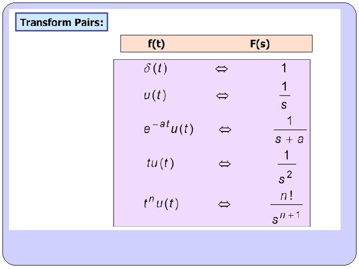
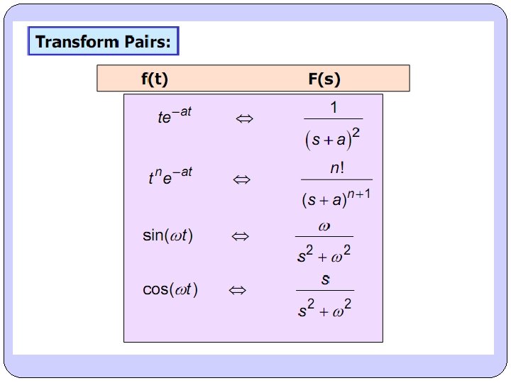
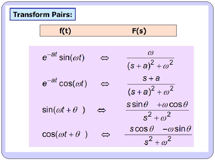
The algorithm for solving transient circuits using Laplace transform • We determine the initial conditions of the circuit (current through the inductors, voltages on capacitors) before switching action. • We draw the equivalent operational circuit, containing the Laplace transform of given sources, the sources corresponding to initial conditions, operational impedances corresponding to the R, L, C elements. • We calculate the images of the given time variable functions (usually voltage of current sources) using direct transformation formula or transform pairs tables. The expressions will depend on the complex variable s.
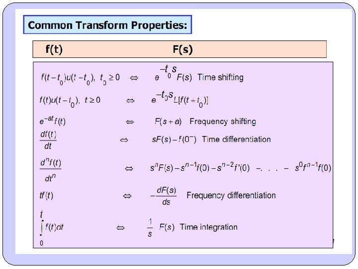
• We apply the operational expresions of Kirchhoff Equations (or different methods ussually applied to circuits: loop method, node potentials methods, etc). These equations will be solved with respect to Laplace images of the unknown functions. • After finding the Laplace transforms of the unknown quantities, the original functions (time dependent) are determined using inversion methods (Mellin-Fourier, Heaviside formulas or tables with transform pairs);
Example 1 Let’s consider the circuit given in Fig. 1 -a, with the following values of the circuit elements : R 1 = 6 , R 2 = 3 , inductance L = 0. 8 m. H, and constant value of the input voltage source E = 36 V. At moment t =0 the switch K closes. Using Laplace transform method determine the variations of the currents through the three elements of circuit and variation of the inductor voltage. Fig. 1 -a
Fig. 1 -b The initial condition of the circuit is determined by the current through the inductor and it can be easily calculated from the circuit presented in the Fig. 1 -b: i L(0–) = 0
After switching (closing K), the equivalent operational circuit is given in the Fig. 1 -c Equivalent circuit after switching Taking into consideration the equivalent circuit, we can determine the total equivalent operational impedance and, then, using Kirchhoff II Theorem, we can calculate the current through the resistor R 1.
Using current divider formula, we can determine the current through resistor R 2, respectively through the inductor L:
In order to determine the voltage on the inductor, we apply Ohm’s law on the respective branch: The original (time dependent functions) are calculated using Heaviside II formula for currents i 1 and i. L, respectively Heaviside I formula for current i 2 and voltage u. L:
; ; ; Replacing also the numerical values, the final solution is:
The representations of these functions with respect to the time , is presented in the Fig. 1 -d, respectively Fig. 1 -e Fig. 1 -d The variation of the circuit currents
t is the time-constant of the circuit: Fig. 1 -e The variation of of the inductor voltage
Example 2 Let’s consider the circuit given in Fig. 2 -a, with the following values of the circuit elements: R = 5 , capacitance C = 1 m. F and constant value of the input voltage source E = 20 V. At t =0 the switch K moves from position a to position b. Using Laplace transform method determine the variations of the currents through the capacitor, respectively the voltage drop on this element. Fig. 2 -a
Fig. 2 -b The circuit before changing the position of switch K. The initial condition for the given circuit is determined by the voltage at the terminal of the capacitor, as represented in the Fig. 2 b:
After switching from a to b, the equivalent operational circuit is presented in Fig. 2 -c: Fig 2 -c The circuit after switching from a to b
If we apply Kirchhoff II Theorem on the loop that contains the capacitor, we obtain: and Taking into consideration the operational expressions of the two functions with respect to s, we apply Heaviside I to determine the time variable current, respectively Heaviside II to determine the time variable voltage on the capacitor:
. Hence we obtain the time-domain expressions for the current, respectively voltage on the capacitor: Replacing the numerical values, we obtain:
. Time variations of these two functions are presented in Fig. 2 -d, respectively Fig. 2 -e: Fig. 2 -d Variation with respect to time of current through capacitor
t is the time constant of the circuit: Fig. 2 -e Variation with respect to time of voltage on capacitor
Example 3 Let’s consider the circuit given in Fig. 3 -a, with the following values of the circuit elements: R 1 = R 2 = 1 k , . inductance L 1 = 1 H, capacitance. C 2 = 100 F and constant value of the input voltage source E = 1 k. V. At moment t =0 the switch K closes. Using Laplace transform method determine the variations of the currents through the inductor and of the voltage on the capacitor.
The initial condition for the given circuit is determined by the voltage on the terminals of the capacitor, as represented in the Fig. 2 -b: i. L(0–) = 0; u. C(0–) = E =1000 V After switching (closing K), the circuit is made by two distinctive circuits: the first one includes the voltage source, the resistor R 1 and inductor L 2, the second includes the resistor R 2 and capacitor C 2.
Fig. 3 -c presents the circuit after switching and the equivalent operational circuits: Fig. 3 -c
Using Kirchhoff II on the respective loops, we can easily calculate the Laplace images of the current through the inductor and the voltage on the capacitor. From the Laplace expression of the current (that was decomposed using partial fractions) we deduce the original function (timevariable current):
In order to determine the voltage on the capacitor we have to calculate firstly the current through the loop IC(s) and then, taking into consideration Kirchhoff II applied on the loop, the voltage can be written as: UC(s) = R 2 IC(s).
The time variations of the current and voltage are represented in the figures Fig. 3 -d, respectively Fig. 3 -e. Fig. 3 -d
Fig. 3 -e
BIBLIOGRAPHY: • Norman Balabanian: Electric Circuits; Mc. Graw. Hill, Inc. , USA, 1994 • K. E. Holbert: Laplace transform solutions of ODE’s, 2006 • Walter Green: The Laplace transform presentation; University of Tennessee, Electrical and Computer Engineering Dep. Knoxville, Tennessee • E. Cazacu, O. Drosu, G. Epureanu, Theory and applications of electric circuits: vol. 1 Transient state analysis Matrix Rom, Bucharest, 2005.