Languages and Compilers SProg og Oversttere Compiler Optimizations

Languages and Compilers (SProg og Oversættere) Compiler Optimizations Bent Thomsen Department of Computer Science Aalborg University With acknowledgement to Norm Hutchinson and Mooly Sagiv whose slides this lecture is based on. 1

Compiler Optimizations The code generated by the Mini. Triangle compiler is not efficient: • We did some optimizations by special code templates, but – It still computes some values at runtime that could be known at compile time – It still computes values more times than necessary – It produces code that will never be executed We can do better! We can do code transformations • Code transformations are performed for a variety of reasons among which are: – To reduce the size of the code – To reduce the running time of the program – To take advantage of machine idioms • Code optimizations include: – – Constant folding Common sub-expression elimination Code motion Dead code elimination • Mathematically, the generation of optimal code is undecideable. 2

Criteria for code-improving transformations • Preserve meaning of programs (safety) – Potentially unsafe transformations • Associative reorder of operands • Movement of expressions and code sequences • Loop unrolling • Must be worth the effort (profitability) and – on average, speed up programs • 90/10 Rule: Programs spend 90% of their execution time in 10% of the code. Identify and improve "hot spots" rather than trying to improve everything. 3

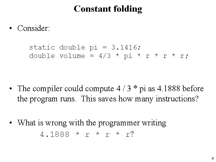
Constant folding • Consider: static double pi = 3. 1416; double volume = 4/3 * pi * r * r; • The compiler could compute 4 / 3 * pi as 4. 1888 before the program runs. This saves how many instructions? • What is wrong with the programmer writing 4. 1888 * r * r? 4

Constant folding II • Consider: struct { int y, m, d; } holidays[6]; holidays[2]. m = 12; holidays[2]. d = 25; • If the address of holidays is x, what is the address of holidays[2]. m? • Could the programmer evaluate this at compile time? Safely? 5

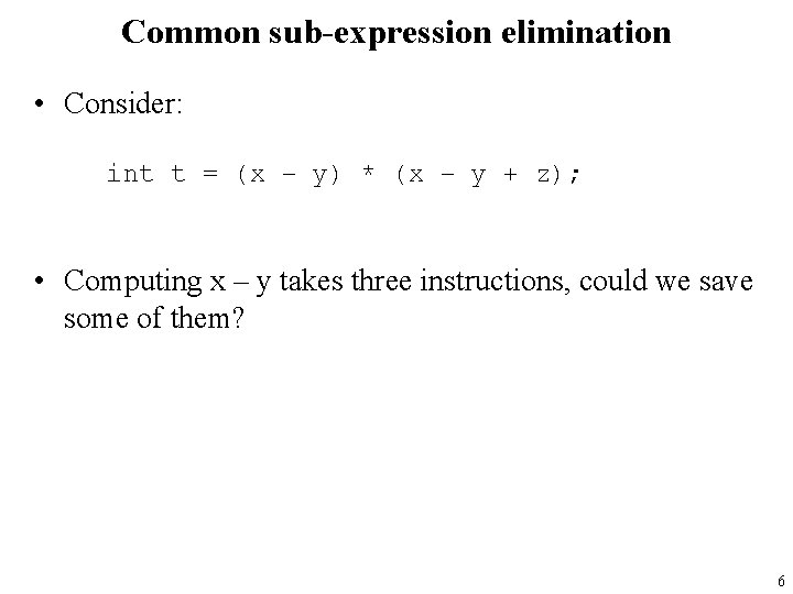
Common sub-expression elimination • Consider: int t = (x – y) * (x – y + z); • Computing x – y takes three instructions, could we save some of them? 6

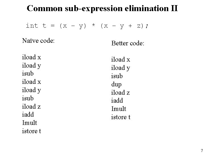
Common sub-expression elimination II int t = (x – y) * (x – y + z); Naïve code: Better code: iload x iload y isub iload z iadd Imult istore t iload x iload y isub dup iload z iadd Imult istore t 7

Common sub-expression elimination III • Consider: struct { int y, m, d; } holidays[6]; holidays[i]. m = 12; holidays[i]. d = 25; • The address of holidays[i] is a common subexpression. 8

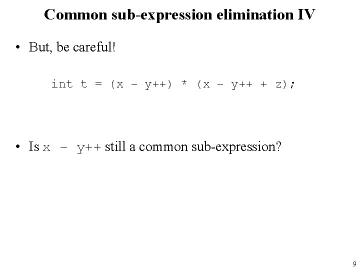
Common sub-expression elimination IV • But, be careful! int t = (x – y++) * (x – y++ + z); • Is x – y++ still a common sub-expression? 9

Code motion • Consider: char name[3][10]; for (int i = 0; i < 3; i++) { for (int j = 0; j < 10; j++) { name[i][j] = ‘a’; • Computing the address of name[i][j] is address[name] + (i * 10) + j • Most of that computation is constant throughout the inner loop address[name] + (i * 10) 10

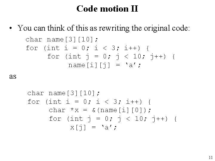
Code motion II • You can think of this as rewriting the original code: char name[3][10]; for (int i = 0; i < 3; i++) { for (int j = 0; j < 10; j++) { name[i][j] = ‘a’; as char name[3][10]; for (int i = 0; i < 3; i++) { char *x = &(name[i][0]); for (int j = 0; j < 10; j++) { x[j] = ‘a’; 11

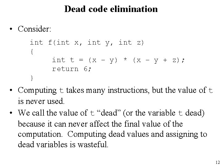
Dead code elimination • Consider: int f(int x, int y, int z) { int t = (x – y) * (x – y + z); return 6; } • Computing t takes many instructions, but the value of t is never used. • We call the value of t “dead” (or the variable t dead) because it can never affect the final value of the computation. Computing dead values and assigning to dead variables is wasteful. 12

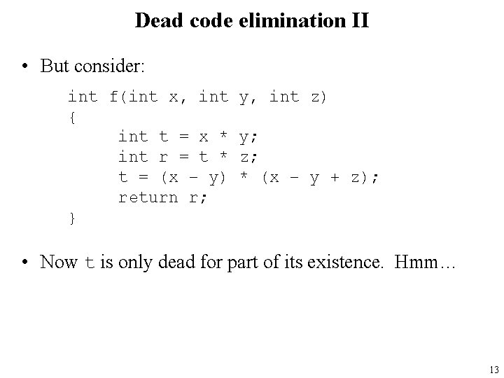
Dead code elimination II • But consider: int f(int x, int { int t = x * int r = t * t = (x – y) return r; } y, int z) y; z; * (x – y + z); • Now t is only dead for part of its existence. Hmm… 13

Optimization implementation • What do we need to know in order to apply an optimization? –Constant folding –Common sub-expression elimination –Code motion –Dead code elimination • Is the optimization correct or safe? • Is the optimization an improvement? • What sort of analyses do we need to perform to get the required information? 14

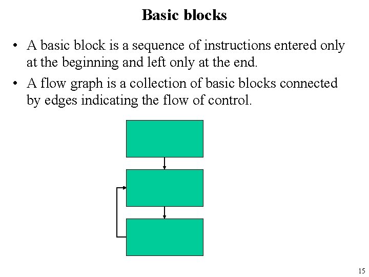
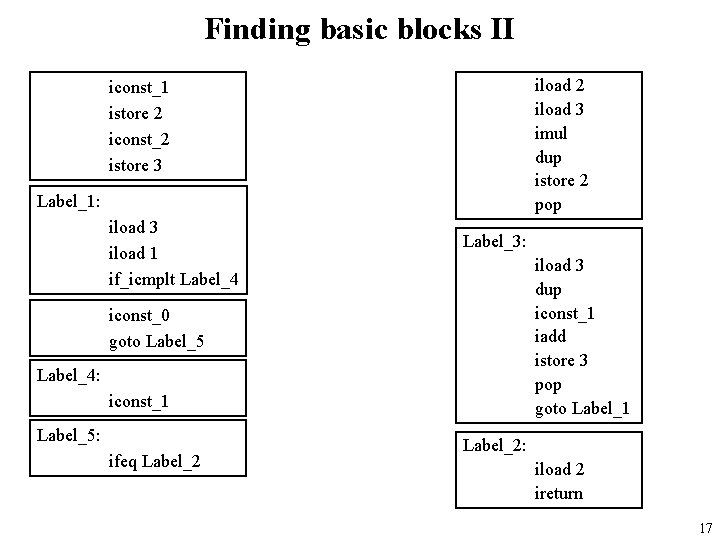
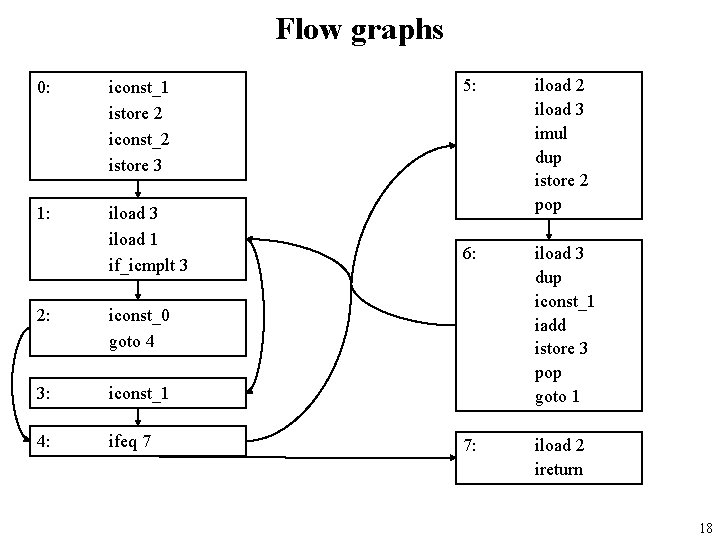
Basic blocks • A basic block is a sequence of instructions entered only at the beginning and left only at the end. • A flow graph is a collection of basic blocks connected by edges indicating the flow of control. 15

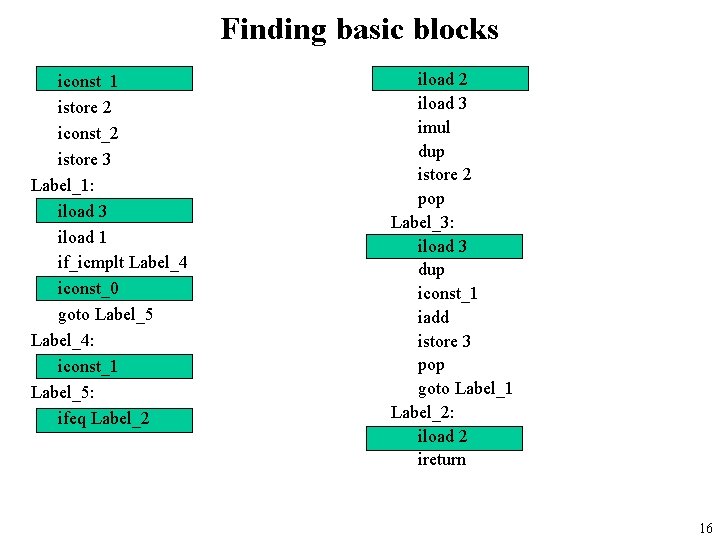
Finding basic blocks iconst_1 istore 2 iconst_2 istore 3 Label_1: iload 3 iload 1 if_icmplt Label_4 iconst_0 goto Label_5 Label_4: iconst_1 Label_5: ifeq Label_2 iload 3 imul dup istore 2 pop Label_3: iload 3 dup iconst_1 iadd istore 3 pop goto Label_1 Label_2: iload 2 ireturn 16

Finding basic blocks II iload 2 iload 3 imul dup istore 2 pop iconst_1 istore 2 iconst_2 istore 3 Label_1: iload 3 iload 1 if_icmplt Label_4 Label_3: iload 3 dup iconst_1 iadd istore 3 pop goto Label_1 iconst_0 goto Label_5 Label_4: iconst_1 Label_5: ifeq Label_2: iload 2 ireturn 17

Flow graphs 0: iconst_1 istore 2 iconst_2 istore 3 1: iload 3 iload 1 if_icmplt 3 2: iconst_0 goto 4 3: iconst_1 4: ifeq 7 5: iload 2 iload 3 imul dup istore 2 pop 6: iload 3 dup iconst_1 iadd istore 3 pop goto 1 7: iload 2 ireturn 18

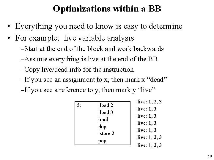
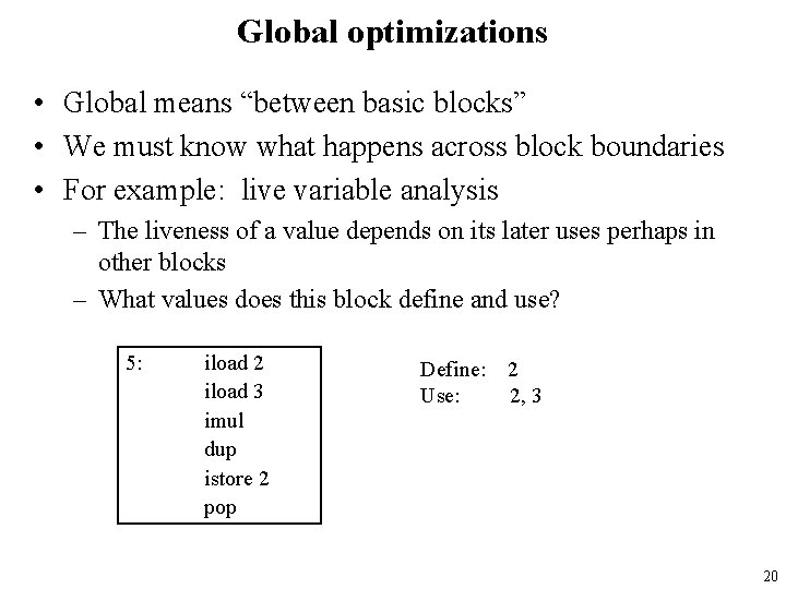
Optimizations within a BB • Everything you need to know is easy to determine • For example: live variable analysis –Start at the end of the block and work backwards –Assume everything is live at the end of the BB –Copy live/dead info for the instruction –If you see an assignment to x, then mark x “dead” –If you see a reference to y, then mark y “live” 5: iload 2 iload 3 imul dup istore 2 pop live: 1, 2, 3 live: 1, 3 live: 1, 2, 3 19

Global optimizations • Global means “between basic blocks” • We must know what happens across block boundaries • For example: live variable analysis – The liveness of a value depends on its later uses perhaps in other blocks – What values does this block define and use? 5: iload 2 iload 3 imul dup istore 2 pop Define: 2 Use: 2, 3 20

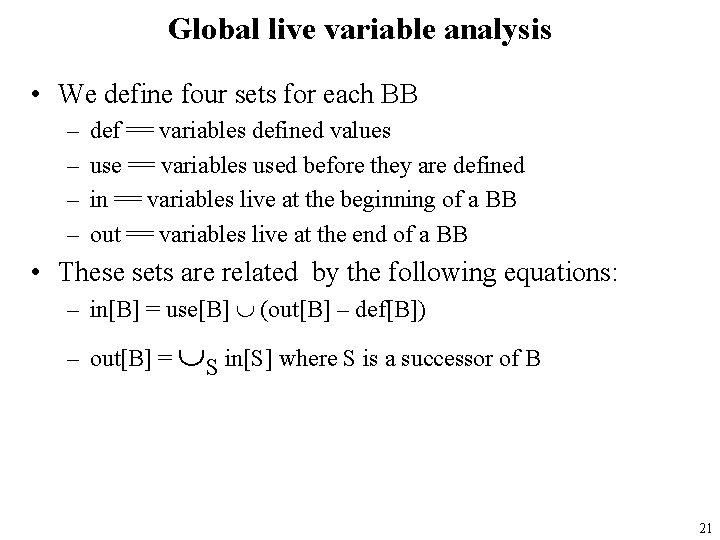
Global live variable analysis • We define four sets for each BB – – def == variables defined values use == variables used before they are defined in == variables live at the beginning of a BB out == variables live at the end of a BB • These sets are related by the following equations: – in[B] = use[B] (out[B] – def[B]) – out[B] = S in[S] where S is a successor of B 21

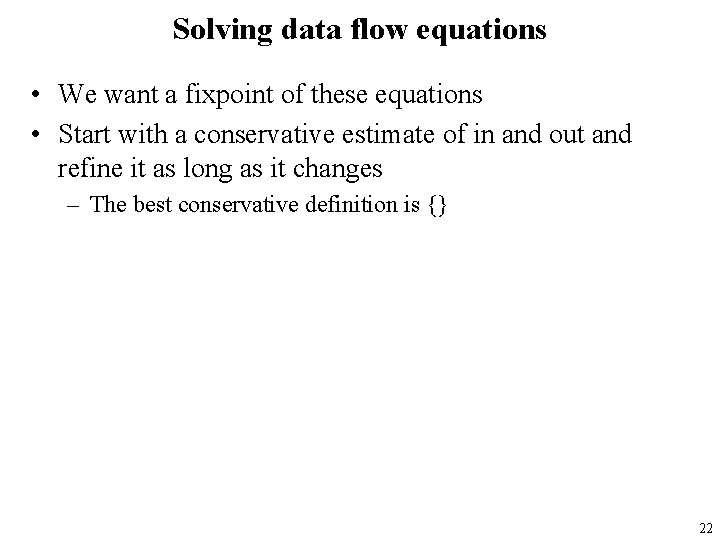
Solving data flow equations • We want a fixpoint of these equations • Start with a conservative estimate of in and out and refine it as long as it changes – The best conservative definition is {} 22

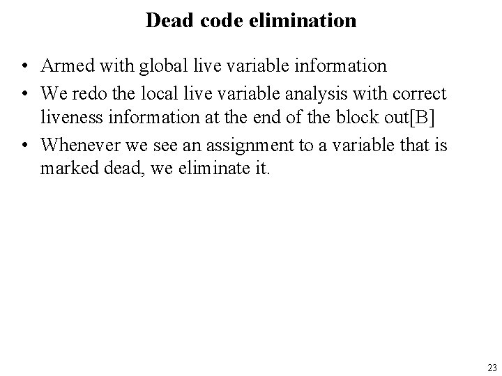
Dead code elimination • Armed with global live variable information • We redo the local live variable analysis with correct liveness information at the end of the block out[B] • Whenever we see an assignment to a variable that is marked dead, we eliminate it. 23

Static Analysis • Automatic derivation of static properties which hold on every execution leading to a program location 24

Example Static Analysis Problems • • • Live variables Reaching definitions Expressions that are “available” Dead code Pointer variables never point into the same location Points in the program in which it is safe to free an object An invocation of virtual method whose address is unique Statements that can be executed in parallel An access to a variable which must be in cache Integer intervals Security properties … 25

Foundation of Static Analysis • Static analysis can be viewed as interpreting the program over an “abstract domain” • Execute the program over larger set of execution paths • Guarantee sound results – Every identified constant is indeed a constant – But not every constant is identified as such 26

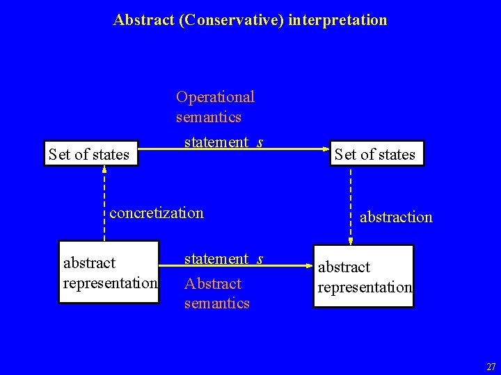
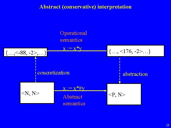
Abstract (Conservative) interpretation Set of states Operational semantics statement s concretization abstract representation statement s Abstract semantics Set of states abstraction abstract representation 27

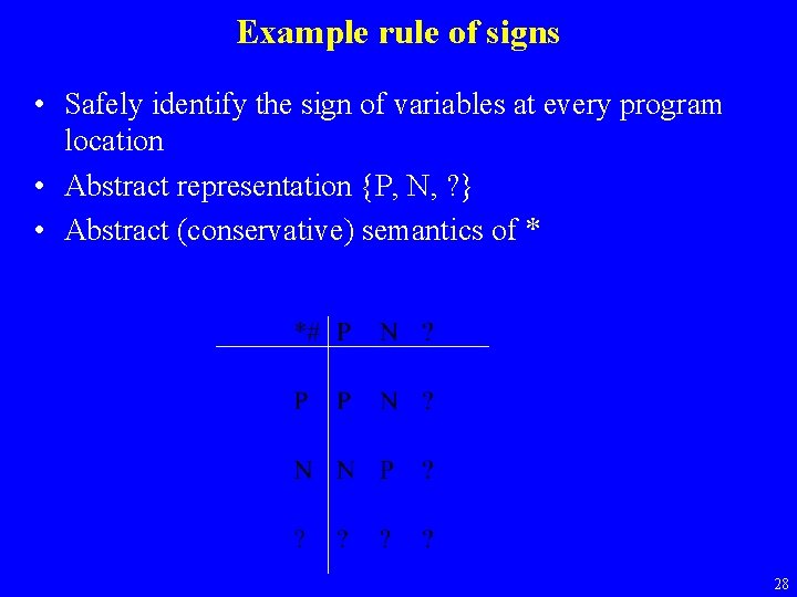
Example rule of signs • Safely identify the sign of variables at every program location • Abstract representation {P, N, ? } • Abstract (conservative) semantics of * 28

Abstract (conservative) interpretation {…, <-88, -2>, …} Operational semantics x : = x*y concretization <N, N> x : = x*#y Abstract semantics {…, <176, -2>…} abstraction <P, N> 29

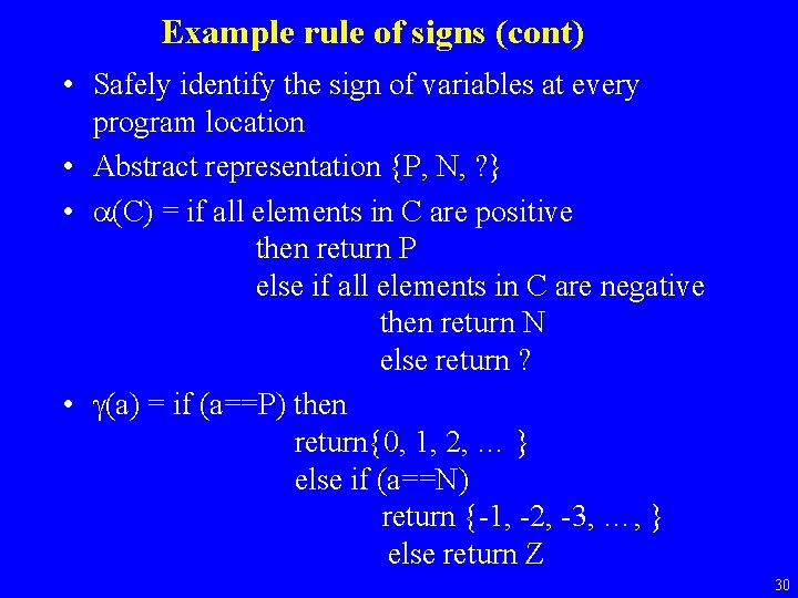
Example rule of signs (cont) • Safely identify the sign of variables at every program location • Abstract representation {P, N, ? } • (C) = if all elements in C are positive then return P else if all elements in C are negative then return N else return ? • (a) = if (a==P) then return{0, 1, 2, … } else if (a==N) return {-1, -2, -3, …, } else return Z 30

Undecidability Issues • It is undecidable if a program point is reachable in some execution • Some static analysis problems are undecidable even if the program conditions are ignored 31

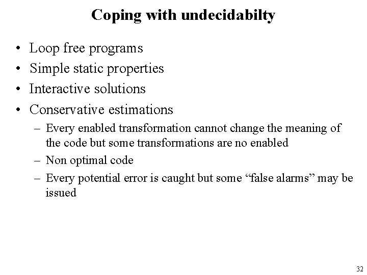
Coping with undecidabilty • • Loop free programs Simple static properties Interactive solutions Conservative estimations – Every enabled transformation cannot change the meaning of the code but some transformations are no enabled – Non optimal code – Every potential error is caught but some “false alarms” may be issued 32

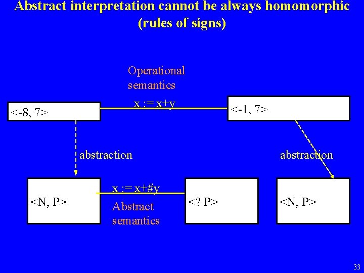
Abstract interpretation cannot be always homomorphic (rules of signs) <-8, 7> Operational semantics x : = x+y <-1, 7> abstraction <N, P> x : = x+#y Abstract semantics abstraction <? P> <N, P> 33

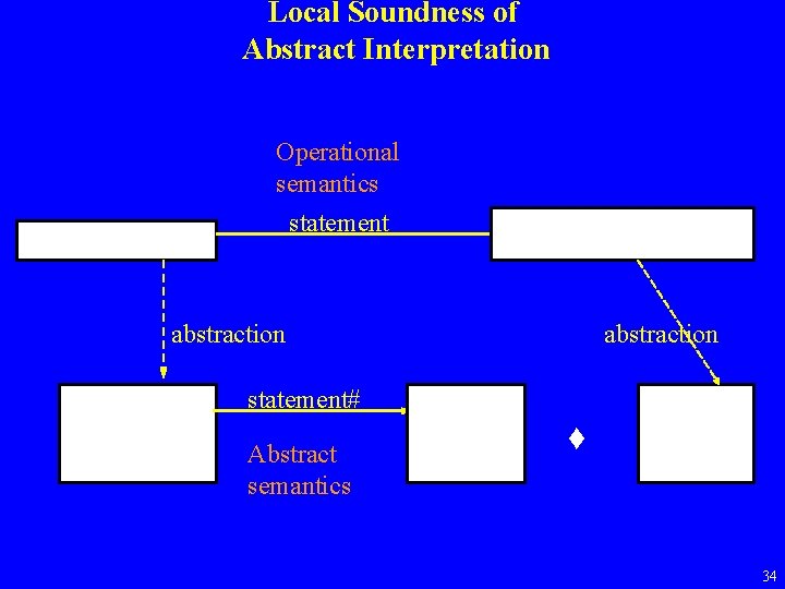
Local Soundness of Abstract Interpretation Operational semantics statement abstraction statement# Abstract semantics 34

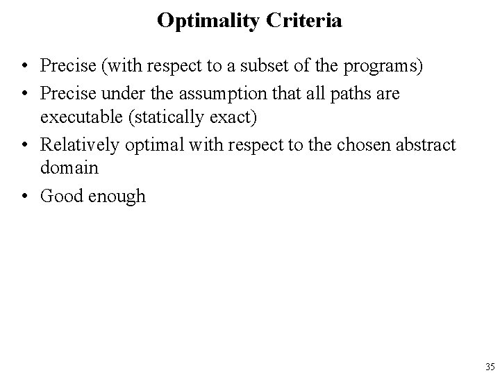
Optimality Criteria • Precise (with respect to a subset of the programs) • Precise under the assumption that all paths are executable (statically exact) • Relatively optimal with respect to the chosen abstract domain • Good enough 35

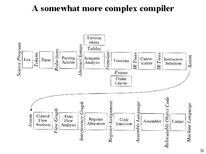
A somewhat more complex compiler 36

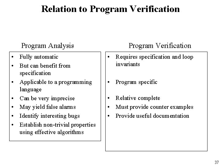
Relation to Program Verification Program Analysis • Fully automatic • But can benefit from specification • Applicable to a programming language • Can be very imprecise • May yield false alarms • Identify interesting bugs • Establish non-trivial properties using effective algorithms Program Verification • Requires specification and loop invariants • Program specific • Relative complete • Must provide counter examples • Provide useful documentation 37

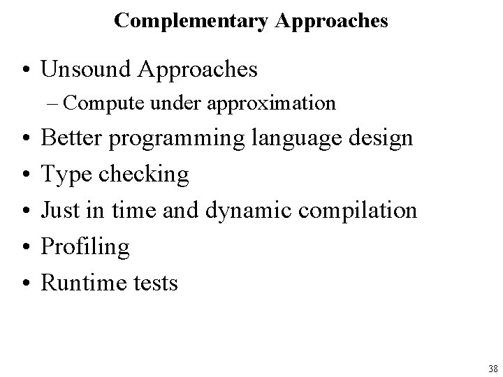
Complementary Approaches • Unsound Approaches – Compute under approximation • • • Better programming language design Type checking Just in time and dynamic compilation Profiling Runtime tests 38