Language Models for Information Retrieval Berlin Chen Department

Language Models for Information Retrieval Berlin Chen Department of Computer Science & Information Engineering National Taiwan Normal University References: 1. W. B. Croft and J. Lafferty (Editors). Language Modeling for Information Retrieval. July 2003 2. T. Hofmann. Unsupervised Learning by Probabilistic Latent Semantic Analysis. Machine Learning, January. February 2001 3. Christopher D. Manning, Prabhakar Raghavan and Hinrich Schütze, Introduction to Information Retrieval, Cambridge University Press, 2008. (Chapter 12) 4. D. A. Grossman, O. Frieder, Information Retrieval: Algorithms and Heuristics, Springer, 2004 (Chapter 2)

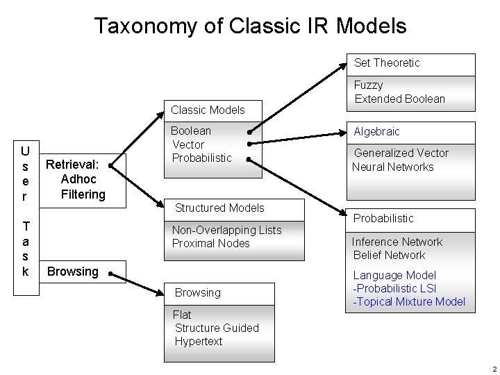
Taxonomy of Classic IR Models Set Theoretic Classic Models U s e r T a s k Retrieval: Adhoc Filtering Boolean Vector Probabilistic Structured Models Non-Overlapping Lists Proximal Nodes Browsing Fuzzy Extended Boolean Algebraic Generalized Vector Neural Networks Probabilistic Inference Network Belief Network Language Model -Probabilistic LSI -Topical Mixture Model Flat Structure Guided Hypertext 2

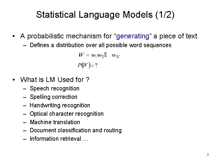
Statistical Language Models (1/2) • A probabilistic mechanism for “generating” a piece of text – Defines a distribution over all possible word sequences • What is LM Used for ? – – – – Speech recognition Spelling correction Handwriting recognition Optical character recognition Machine translation Document classification and routing Information retrieval … 3

Statistical Language Models (2/2) • (Statistical) language models (LM) have been widely used for speech recognition and language (machine) translation for more than twenty years • However, their use for information retrieval started only in 1998 [Ponte and Croft, SIGIR 1998] 4

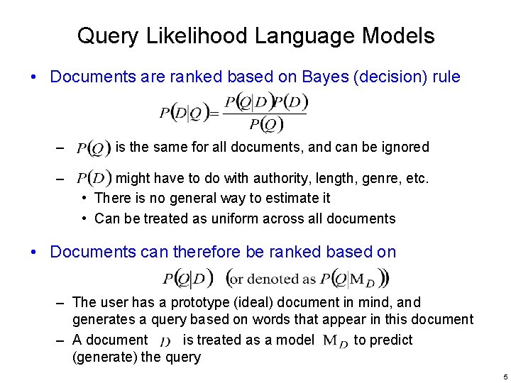
Query Likelihood Language Models • Documents are ranked based on Bayes (decision) rule – is the same for all documents, and can be ignored – might have to do with authority, length, genre, etc. • There is no general way to estimate it • Can be treated as uniform across all documents • Documents can therefore be ranked based on – The user has a prototype (ideal) document in mind, and generates a query based on words that appear in this document – A document is treated as a model to predict (generate) the query 5

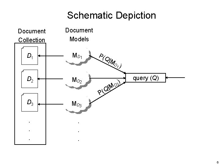
Schematic Depiction Document Collection Document Models D 1 MD 1 P(Q |M D ) 1 D 2 MD 2 P( D 3 MD 3 . . . MD | Q ) 3 query (Q) 6

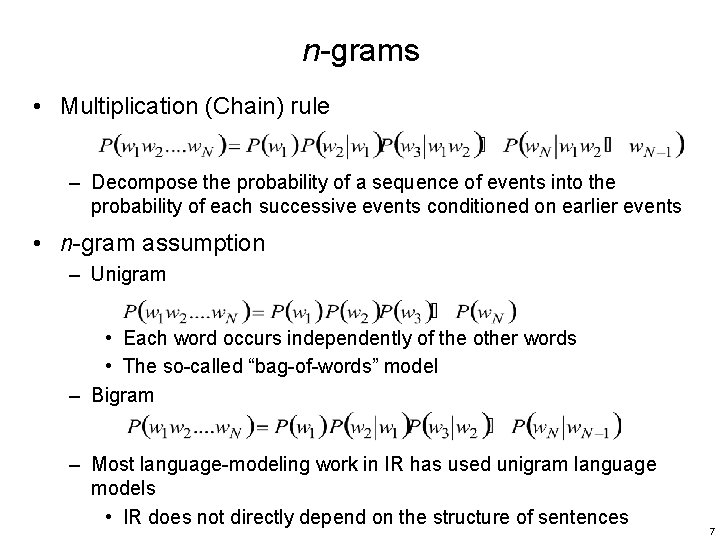
n-grams • Multiplication (Chain) rule – Decompose the probability of a sequence of events into the probability of each successive events conditioned on earlier events • n-gram assumption – Unigram • Each word occurs independently of the other words • The so-called “bag-of-words” model – Bigram – Most language-modeling work in IR has used unigram language models • IR does not directly depend on the structure of sentences 7

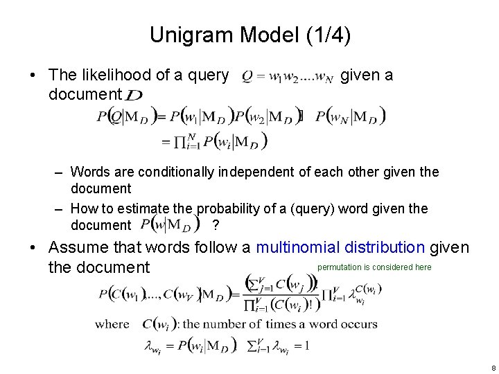
Unigram Model (1/4) • The likelihood of a query document given a – Words are conditionally independent of each other given the document – How to estimate the probability of a (query) word given the document ? • Assume that words follow a multinomial distribution given permutation is considered here the document 8

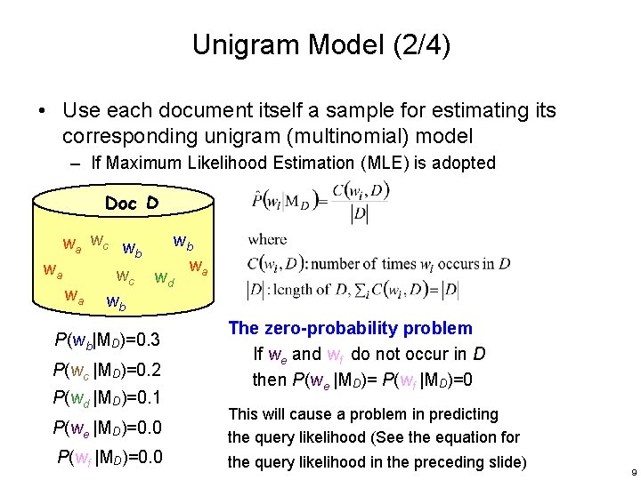
Unigram Model (2/4) • Use each document itself a sample for estimating its corresponding unigram (multinomial) model – If Maximum Likelihood Estimation (MLE) is adopted Doc D wa wc wb wa wa wc wb wb wa wd P(wb|MD)=0. 3 P(wc |MD)=0. 2 P(wd |MD)=0. 1 The zero-probability problem If we and wf do not occur in D then P(we |MD)= P(wf |MD)=0 P(we |MD)=0. 0 This will cause a problem in predicting the query likelihood (See the equation for P(wf |MD)=0. 0 the query likelihood in the preceding slide) 9

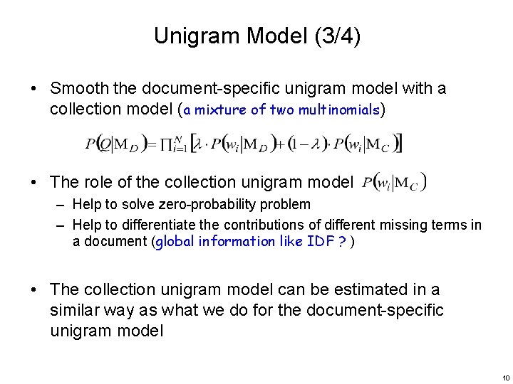
Unigram Model (3/4) • Smooth the document-specific unigram model with a collection model (a mixture of two multinomials) • The role of the collection unigram model – Help to solve zero-probability problem – Help to differentiate the contributions of different missing terms in a document (global information like IDF ? ) • The collection unigram model can be estimated in a similar way as what we do for the document-specific unigram model 10

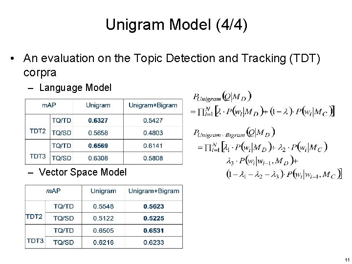
Unigram Model (4/4) • An evaluation on the Topic Detection and Tracking (TDT) corpra – Language Model – Vector Space Model 11

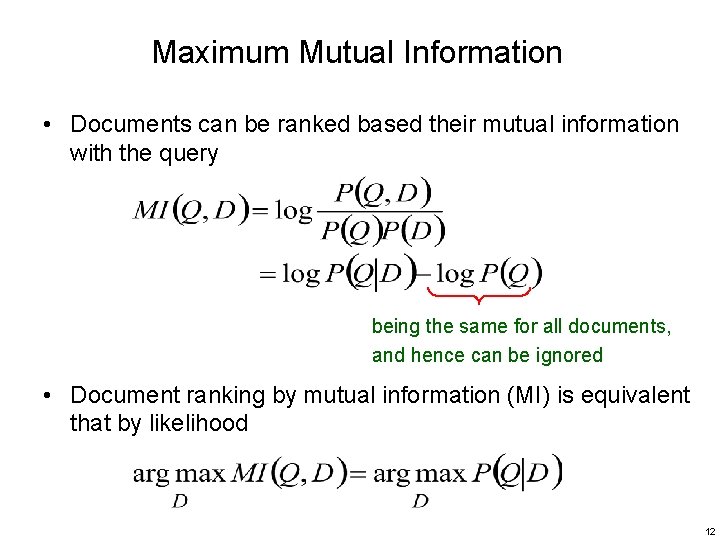
Maximum Mutual Information • Documents can be ranked based their mutual information with the query being the same for all documents, and hence can be ignored • Document ranking by mutual information (MI) is equivalent that by likelihood 12

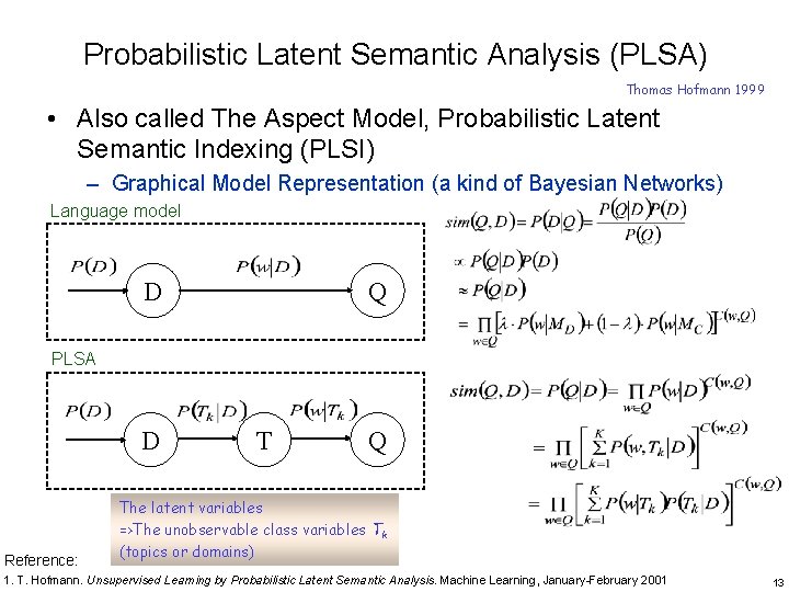
Probabilistic Latent Semantic Analysis (PLSA) Thomas Hofmann 1999 • Also called The Aspect Model, Probabilistic Latent Semantic Indexing (PLSI) – Graphical Model Representation (a kind of Bayesian Networks) Language model Q D PLSA D Reference: T Q The latent variables =>The unobservable class variables Tk (topics or domains) 1. T. Hofmann. Unsupervised Learning by Probabilistic Latent Semantic Analysis. Machine Learning, January-February 2001 13

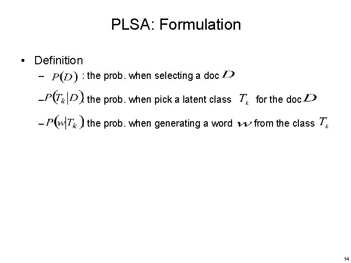
PLSA: Formulation • Definition – : the prob. when selecting a doc – : the prob. when pick a latent class for the doc – : the prob. when generating a word from the class 14

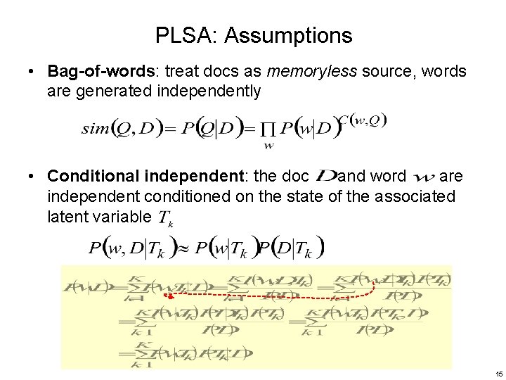
PLSA: Assumptions • Bag-of-words: treat docs as memoryless source, words are generated independently • Conditional independent: the doc and word are independent conditioned on the state of the associated latent variable 15

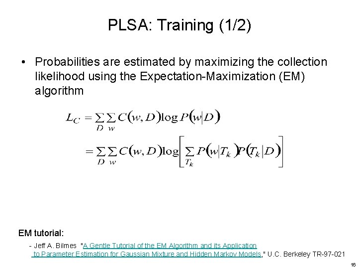
PLSA: Training (1/2) • Probabilities are estimated by maximizing the collection likelihood using the Expectation-Maximization (EM) algorithm EM tutorial: - Jeff A. Bilmes "A Gentle Tutorial of the EM Algorithm and its Application to Parameter Estimation for Gaussian Mixture and Hidden Markov Models, " U. C. Berkeley TR-97 -021 16

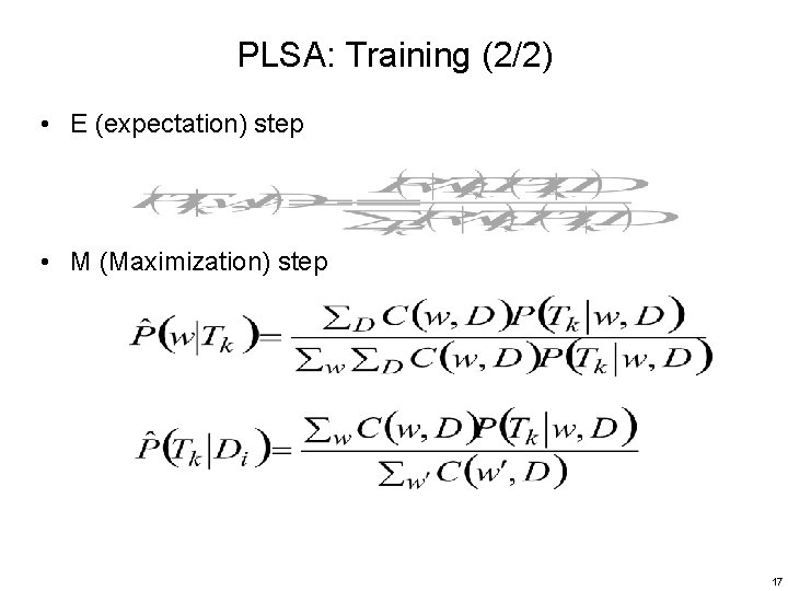
PLSA: Training (2/2) • E (expectation) step • M (Maximization) step 17

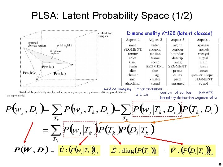
PLSA: Latent Probability Space (1/2) Dimensionality K=128 (latent classes) medical imaging = . image sequence phonetic context of contour analysis boundary detection segmentation . 18

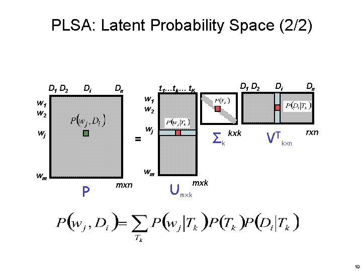
PLSA: Latent Probability Space (2/2) D 1 D 2 Di Dn w 1 w 2 wj wj = D 1 D 2 t 1…tk… t. K Σk kxk Di VT Dn rxn kxn wm wm P mxn mxk Umxk 19

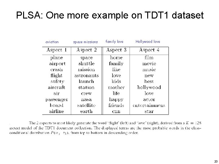
PLSA: One more example on TDT 1 dataset aviation space missions family love Hollywood love 20

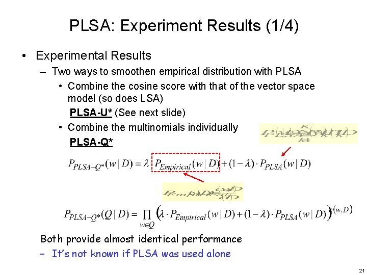
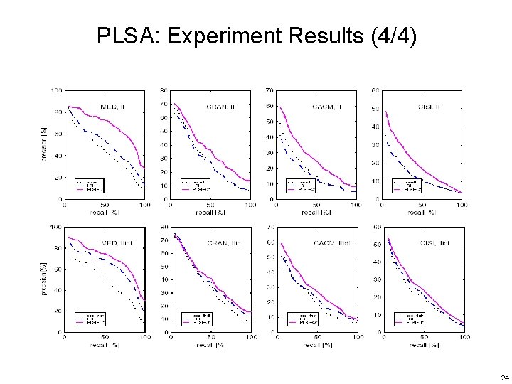
PLSA: Experiment Results (1/4) • Experimental Results – Two ways to smoothen empirical distribution with PLSA • Combine the cosine score with that of the vector space model (so does LSA) PLSA-U* (See next slide) • Combine the multinomials individually PLSA-Q* Both provide almost identical performance – It’s not known if PLSA was used alone 21

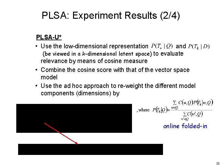
PLSA: Experiment Results (2/4) PLSA-U* • Use the low-dimensional representation and (be viewed in a k-dimensional latent space) to evaluate relevance by means of cosine measure • Combine the cosine score with that of the vector space model • Use the ad hoc approach to re-weight the different model components (dimensions) by online folded-in 22

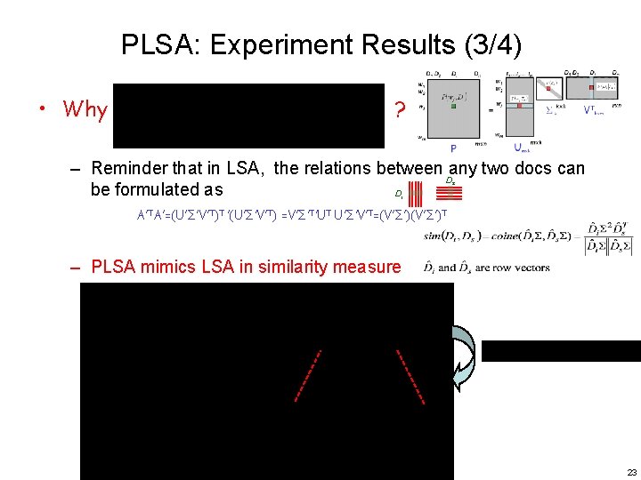
PLSA: Experiment Results (3/4) • Why ? – Reminder that in LSA, the relations between Dany two docs can be formulated as D s i A’TA’=(U’Σ’V’T)T ’(U’Σ’V’T) =V’Σ’T’UT U’Σ’V’T=(V’Σ’)T – PLSA mimics LSA in similarity measure 23

PLSA: Experiment Results (4/4) 24

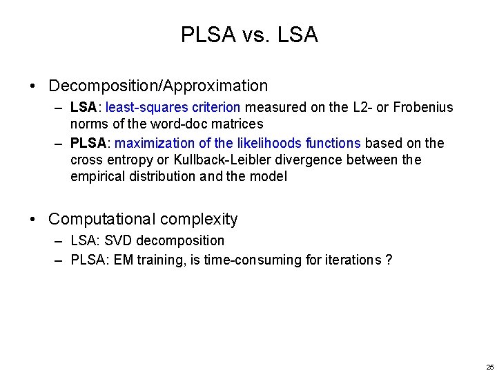
PLSA vs. LSA • Decomposition/Approximation – LSA: least-squares criterion measured on the L 2 - or Frobenius norms of the word-doc matrices – PLSA: maximization of the likelihoods functions based on the cross entropy or Kullback-Leibler divergence between the empirical distribution and the model • Computational complexity – LSA: SVD decomposition – PLSA: EM training, is time-consuming for iterations ? 25