LaneLevel Localization Using an AVM Camera for an

Overview A lane-level localization algorithm based on a map-matching method. Digital map improves vehicle

Structure of Vehicle Localization (1/2) Structure of vehicle localization. 3 Intelligent Systems Lab.

Structure of Vehicle Localization (2/2) Macro-level: navigation system-GPS and proprioceptive sensors. Road-level: radar and

Around View Monitor Four wide-angle cameras set up at on the front, back, left

Regions of Interest Assign line type (lane or stop line, vertical or horizontal line).

Gaussian Filtered by a two dimensional Gaussian kernel. Vertical direction of image A and

Random Sample Consensus After thresholding, RANSAC uses a model with randomly selected edge points

Map-Matching Based on ICP A two-dimensional point-to-plane ICP algorithm matches digital map with the

Matching Covariance Estimation (1/2) Haralick’s method is estimate the ICP’s covariance. The approximate value

Matching Covariance Estimation (2/2) Estimated standard deviation of matching error (red line) and true

Localization Filter Position from ICP : observation inside EKF. Validation gate: solve false matching.

Extended Kalman Filter (1/3) Uk: external input (velocity and yaw-rate) Zk: corrected vehicle position.

Extended Kalman Filter (2/3) Nominal discrete process model equation estimated states from previous time

Extended Kalman Filter (3/3) Vehicle positions are corrected by a measurement update of the

Validation Gate Prevent fusing the result of false matching. Threshold about acceptability of measurements.

Experimental results (1/7) Lane-level map: RTK-DGPS. accuracy centimeter. Detailed trajectory and travel time on

Experimental results (2/7) Localization result of ﬁrst scenario. (a)lateral position error, (b) longitudinal position

Experimental results (3/7) Localization result of second scenario. (a)lateral position error, (b) longitudinal position

Experimental results (4/7) Operation of map-matching according to the driving maneuvers. 20 Intelligent Systems

Experimental results (5/7) Localization result of second scenario. 21 Intelligent Systems Lab.

Experimental results (6/7) Histogram of the measurement residuals over all datasets. 22 Intelligent Systems

Experimental results (7/7) Compare with method based on the front camera. Lateral accuracy is

Conclusion Lane-level localization using AVM cameras with a lane map is presented. Lane detection

THANK YOU FOR ATTENTION! 25 Intelligent Systems Lab.

Iterative closest point (ICP) It compares the two clouds and finds the transformation matrix

Particle Filter Initial: plenty of particle --X (t), evenly distribute; Prediction: state transition equation--every

Slides: 27

Download presentation

Lane-Level Localization Using an AVM Camera for an Automated Driving Vehicle in Urban Environments Dongwook Kim, Beomjun Kim, Taeyoung Chung, and Kyongsu Yi IEEE/ASME Transactions on Mechatronics, Vol. 22, No. 1, Feb 2017 Presented by: Yang Yu {yuyang@islab. ulsan. ac. kr} Dec. 2, 2017

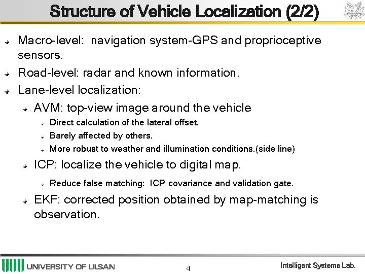
Overview A lane-level localization algorithm based on a map-matching method. Digital map improves vehicle localization. Lane detection: around view monitoring(AVM). Features for map-match: lane marking. Sensor fusion: AVM module and vehicle sensors. Position correction: iterative closest point (ICP). Map matching: map and sensor feature data. Covariance of the ICP is estimated using Haralick’s method. Localization ﬁlter: extended Kalman filter (EKF). 2 Intelligent Systems Lab.

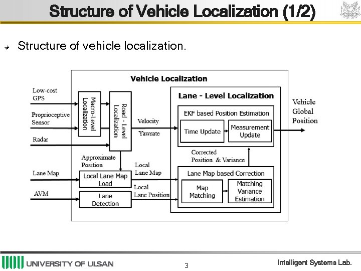
Structure of Vehicle Localization (1/2) Structure of vehicle localization. 3 Intelligent Systems Lab.

Structure of Vehicle Localization (2/2) Macro-level: navigation system-GPS and proprioceptive sensors. Road-level: radar and known information. Lane-level localization: AVM: top-view image around the vehicle Direct calculation of the lateral offset. Barely affected by others. More robust to weather and illumination conditions. (side line) ICP: localize the vehicle to digital map. Reduce false matching: ICP covariance and validation gate. EKF: corrected position obtained by map-matching is observation. 4 Intelligent Systems Lab.

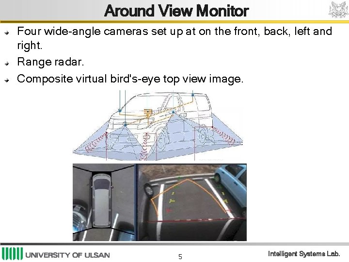
Around View Monitor Four wide-angle cameras set up at on the front, back, left and right. Range radar. Composite virtual bird's-eye top view image. 5 Intelligent Systems Lab.

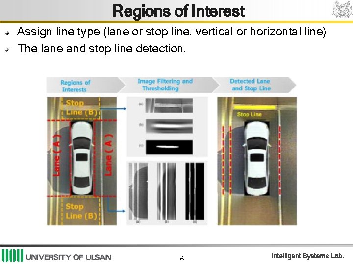
Regions of Interest Assign line type (lane or stop line, vertical or horizontal line). The lane and stop line detection. 6 Intelligent Systems Lab.

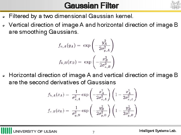
Gaussian Filtered by a two dimensional Gaussian kernel. Vertical direction of image A and horizontal direction of image B are smoothing Gaussians. Horizontal direction of image A and vertical direction of image B are the second derivatives of Gaussians 7 Intelligent Systems Lab.

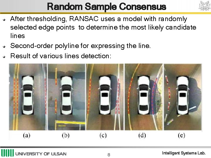
Random Sample Consensus After thresholding, RANSAC uses a model with randomly selected edge points to determine the most likely candidate lines Second-order polyline for expressing the line. Result of various lines detection: 8 Intelligent Systems Lab.

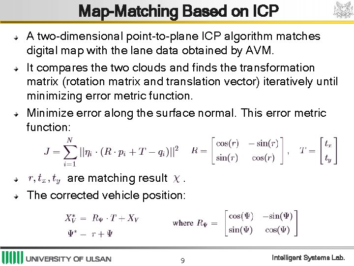
Map-Matching Based on ICP A two-dimensional point-to-plane ICP algorithm matches digital map with the lane data obtained by AVM. It compares the two clouds and finds the transformation matrix (rotation matrix and translation vector) iteratively until minimizing error metric function. Minimize error along the surface normal. This error metric function: are matching result. The corrected vehicle position: 9 Intelligent Systems Lab.

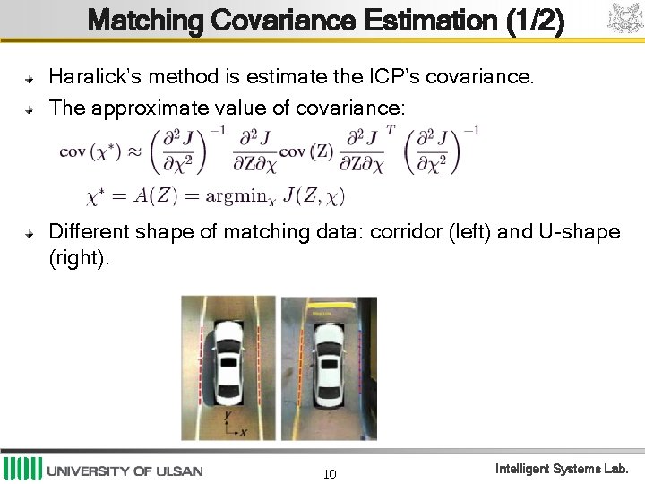
Matching Covariance Estimation (1/2) Haralick’s method is estimate the ICP’s covariance. The approximate value of covariance: Different shape of matching data: corridor (left) and U-shape (right). 10 Intelligent Systems Lab.

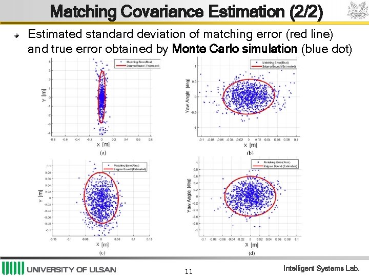
Matching Covariance Estimation (2/2) Estimated standard deviation of matching error (red line) and true error obtained by Monte Carlo simulation (blue dot) 11 Intelligent Systems Lab.

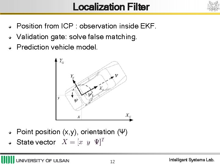
Localization Filter Position from ICP : observation inside EKF. Validation gate: solve false matching. Prediction vehicle model. Point position (x, y), orientation (Ψ) State vector 12 Intelligent Systems Lab.

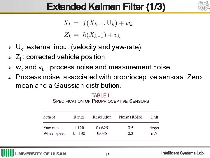
Extended Kalman Filter (1/3) Uk: external input (velocity and yaw-rate) Zk: corrected vehicle position. wk and vk : process noise and measurement noise. Process noise: associated with proprioceptive sensors. Zero mean and a Gaussian distribution. 13 Intelligent Systems Lab.

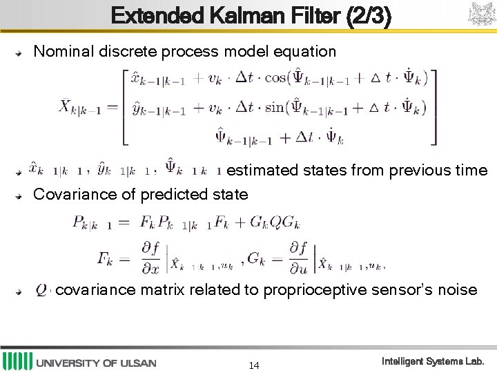
Extended Kalman Filter (2/3) Nominal discrete process model equation estimated states from previous time Covariance of predicted state covariance matrix related to proprioceptive sensor’s noise 14 Intelligent Systems Lab.

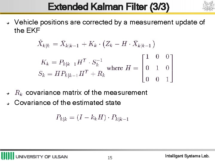
Extended Kalman Filter (3/3) Vehicle positions are corrected by a measurement update of the EKF covariance matrix of the measurement Covariance of the estimated state 15 Intelligent Systems Lab.

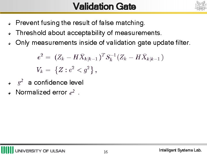
Validation Gate Prevent fusing the result of false matching. Threshold about acceptability of measurements. Only measurements inside of validation gate update ﬁlter. a conﬁdence level Normalized error. 16 Intelligent Systems Lab.

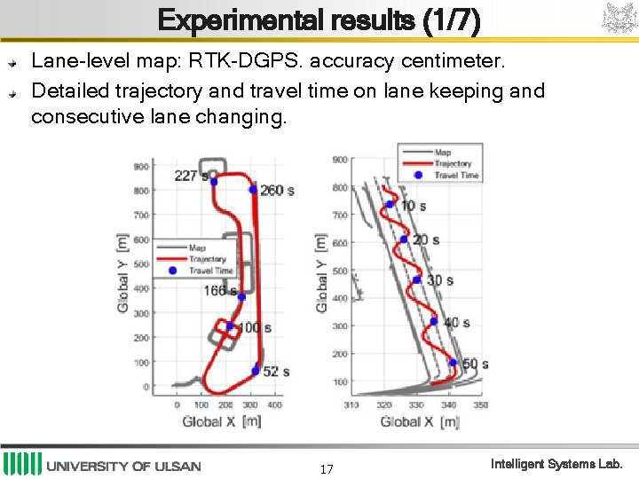
Experimental results (1/7) Lane-level map: RTK-DGPS. accuracy centimeter. Detailed trajectory and travel time on lane keeping and consecutive lane changing. 17 Intelligent Systems Lab.

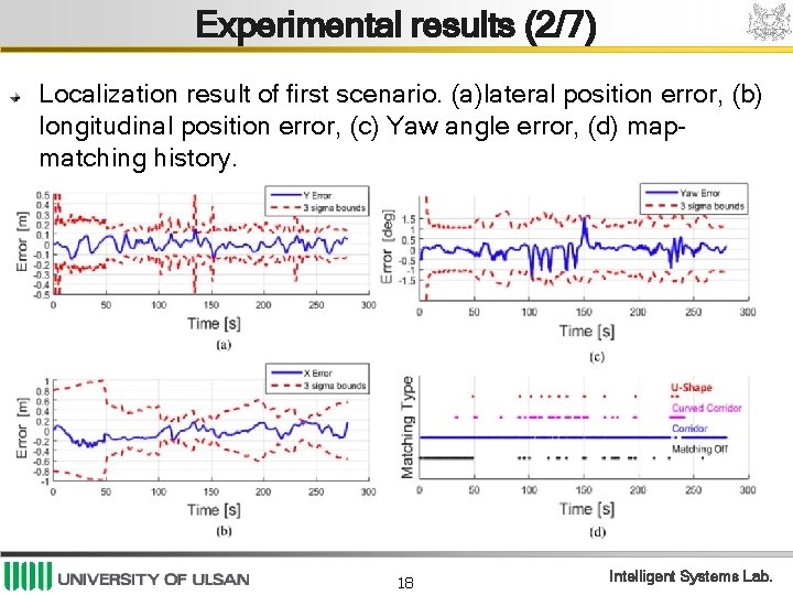
Experimental results (2/7) Localization result of ﬁrst scenario. (a)lateral position error, (b) longitudinal position error, (c) Yaw angle error, (d) mapmatching history. 18 Intelligent Systems Lab.

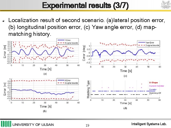
Experimental results (3/7) Localization result of second scenario. (a)lateral position error, (b) longitudinal position error, (c) Yaw angle error, (d) mapmatching history. 19 Intelligent Systems Lab.

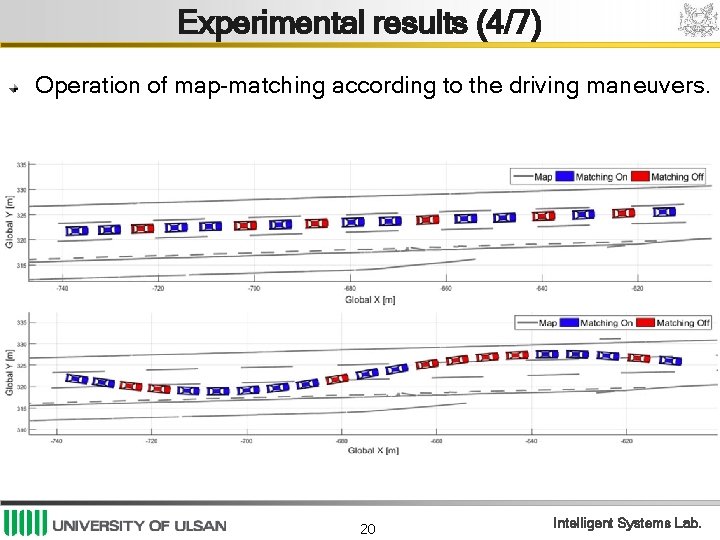
Experimental results (4/7) Operation of map-matching according to the driving maneuvers. 20 Intelligent Systems Lab.

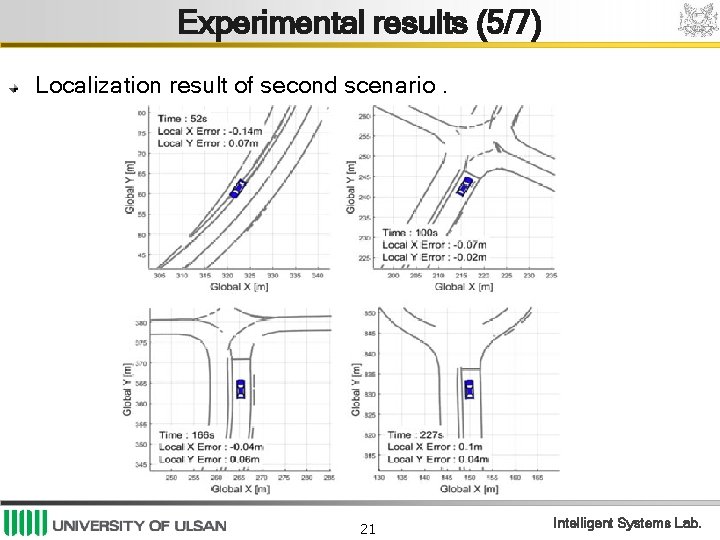
Experimental results (5/7) Localization result of second scenario. 21 Intelligent Systems Lab.

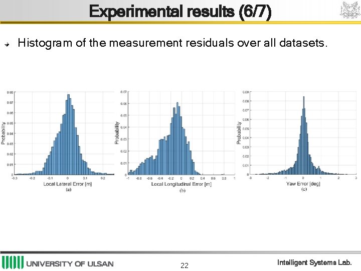
Experimental results (6/7) Histogram of the measurement residuals over all datasets. 22 Intelligent Systems Lab.

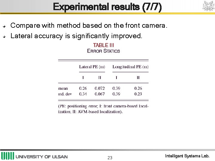
Experimental results (7/7) Compare with method based on the front camera. Lateral accuracy is signiﬁcantly improved. 23 Intelligent Systems Lab.

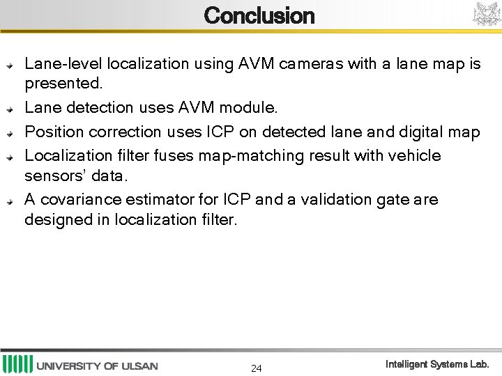
Conclusion Lane-level localization using AVM cameras with a lane map is presented. Lane detection uses AVM module. Position correction uses ICP on detected lane and digital map Localization ﬁlter fuses map-matching result with vehicle sensors’ data. A covariance estimator for ICP and a validation gate are designed in localization ﬁlter. 24 Intelligent Systems Lab.

THANK YOU FOR ATTENTION! 25 Intelligent Systems Lab.

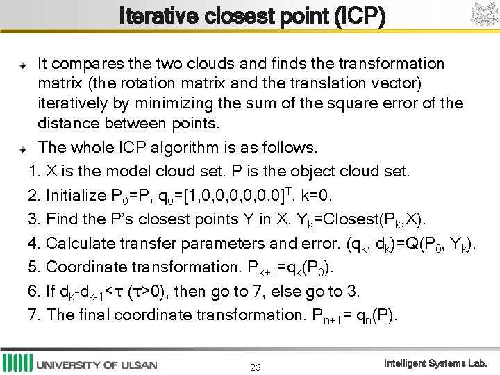
Iterative closest point (ICP) It compares the two clouds and finds the transformation matrix (the rotation matrix and the translation vector) iteratively by minimizing the sum of the square error of the distance between points. The whole ICP algorithm is as follows. 1. X is the model cloud set. P is the object cloud set. 2. Initialize P 0=P, q 0=[1, 0, 0, 0]T, k=0. 3. Find the P’s closest points Y in X. Yk=Closest(Pk, X). 4. Calculate transfer parameters and error. (qk, dk)=Q(P 0, Yk). 5. Coordinate transformation. Pk+1=qk(P 0). 6. If dk-dk-1<τ (τ>0), then go to 7, else go to 3. 7. The final coordinate transformation. Pn+1= qn(P). 26 Intelligent Systems Lab.

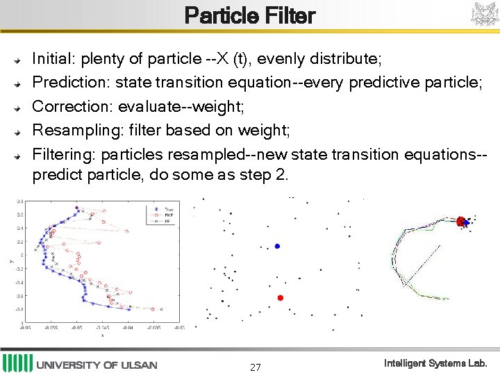
Particle Filter Initial: plenty of particle --X (t), evenly distribute; Prediction: state transition equation--every predictive particle; Correction: evaluate--weight; Resampling: filter based on weight; Filtering: particles resampled--new state transition equations-predict particle, do some as step 2. 27 Intelligent Systems Lab.