Landscape Linkage Modeling Peter Singleton Brad Mc Rae

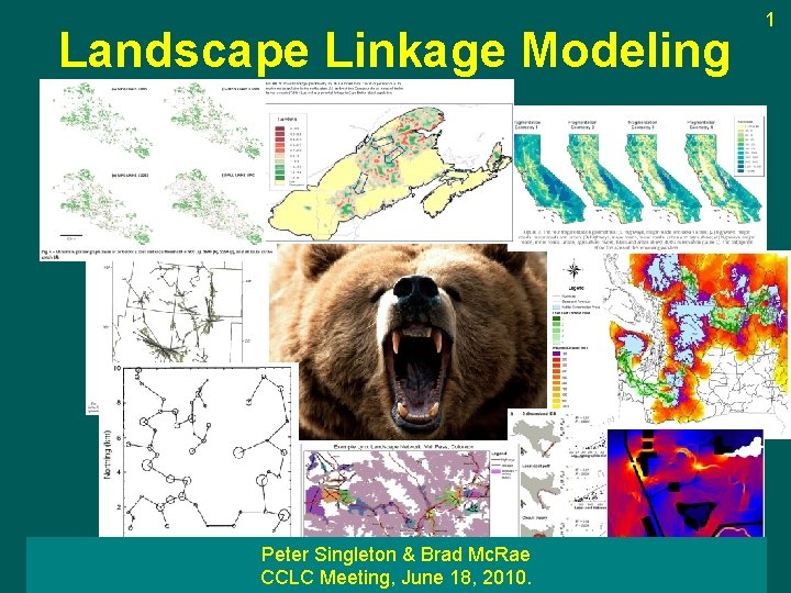
Landscape Linkage Modeling Peter Singleton & Brad Mc. Rae CCLC Meeting, June 18, 2010. 1

Introduction • Landscape Configuration is Important! – Animals need to be able to move at a variety of scales – Intra-territorial movements • Habitat resources need to configured in a way that they are accessible – Inter-territorial movements • Metapopulation function • Dispersal • Range Shifts

2 Introduction Definitions of connectivity: Merriam 1984: The degree to which absolute isolation is prevented by landscape elements which allow organisms to move among patches. Taylor et al 1993: The degree to which the landscape impedes or facilitates movement among resource patches. With et al 1997: The functional relationship among habitat patches owing to the spatial contagion of habitat and the movement responses of organisms to landscape structure. Singleton et al 2002: The quality of a heterogeneous land area to provide for passage of animals (landscape permeability).

Introduction Standard Definitions from Merriam-Webster. com Connectivity: Connect – 1. to join or fasten together usually by something intervening (Latin com- + nectere to bind) Linkage: Link – 1. a connecting structure (Old Norse hlekkr chain) Corridor: 1. a passageway into which compartments or rooms open, 2. an area or narrow stretch of land identified by a specific common characteristic or purpose, 3. a land path used by migrating animals (Italian correre to run) Permeability: Permeate – 1. to diffuse through or penetrate something 2. to pass through the pores of interstices of (Latin permeatus, from per- through + meare to go, pass)

3 Introduction • Structural Connectivity: The spatial arrangement of different types of habitat or other elements in the landscape. • Functional Connectivity: The behavioral response of individuals, species, or ecological processes to the physical structure of the landscape. – Potential Connectivity – Actual Connectivity

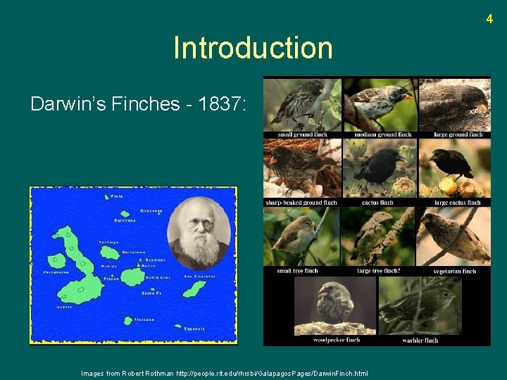
4 Introduction Darwin’s Finches - 1837: Images from Robert Rothman http: //people. rit. edu/rhrsbi/Galapagos. Pages/Darwin. Finch. html

Introduction Island Biography • Mac. Arthur & Wilson 1967 Theory of Island Biogeography Reserve Design • Soule 1987 Viable Populations for Conservation • Meffe & Carroll 1994 Conservation Biology Textbook Conservation Corridors • Servheen & Sandstrom 1993 Linkage Zones for Grizzly Bears… End. Sp. Bul. 18 • Walker & Craighead 1997 Analyzing Wildlife Movement Corridors… Proc. ESRI Users Conf. • Around 2000, linkage assessment workshops start happening • Mid-’ 00’s, lots of publications addressing corridors / connectivity Landscape Processes • Late-’ 00’s Maturation of landscape genetics & modeling techniques • Future? – More empirical data relating landscape process and pattern? – More sophisticated simulation modeling – Address climate change adaptation concerns 5

Introduction • Types of ecological models – Conceptual models • Consistent syntheses of existing information that allow a systematic exploration of the way we think a process works – Statistical models • Based on empirical information – Simulation models • Similar to conceptual models, but provide a more detailed exploration of a specific process

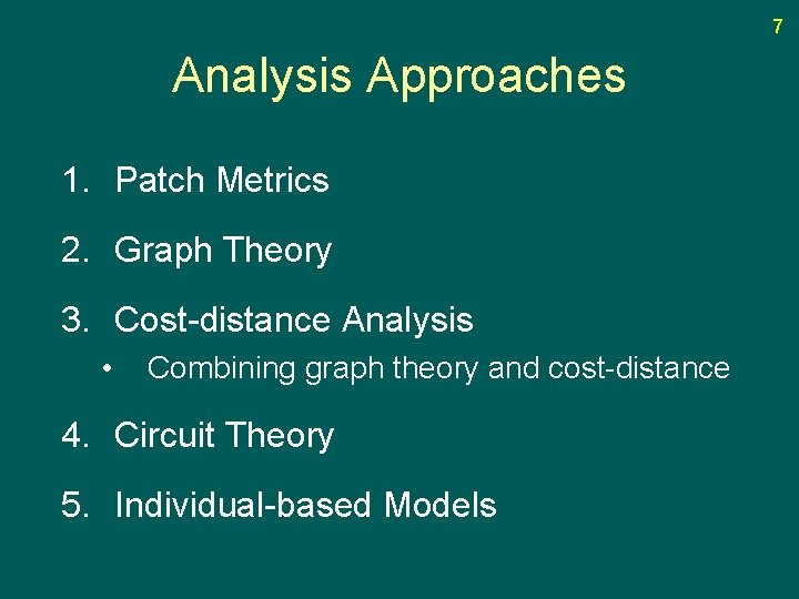
7 Analysis Approaches 1. Patch Metrics 2. Graph Theory 3. Cost-distance Analysis • Combining graph theory and cost-distance 4. Circuit Theory 5. Individual-based Models

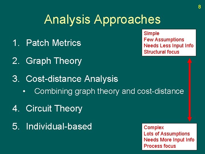
8 Analysis Approaches 1. Patch Metrics Simple Few Assumptions Needs Less Input Info Structural focus 2. Graph Theory 3. Cost-distance Analysis • Combining graph theory and cost-distance 4. Circuit Theory 5. Individual-based Complex Lots of Assumptions Needs More Input Info Process focus

9 Analysis Approaches 1) Patch Metrics • Quantifies Patch Characteristics or Relationships Between Patches (e. g. patch size, nearest neighbor) • Emphasizes Structural Connectivity • Generally must be summarized across a landscape unit (e. g. watershed or planning unit) • Very useful for quantifying landscape patterns (e. g. historic range of variability, monitoring change, comparing landscapes) • Structure, not process oriented • Don’t provide a lot of information about expected movement patterns

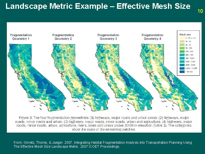
Landscape Metric Example – Effective Mesh Size From: Girvetz, Thorne, & Jaeger. 2007. Integrating Habitat Fragmentation Analysis into Transportation Planning Using The Effective Mesh Size Landscape Metric. 2007 ICOET Proceedings. 10

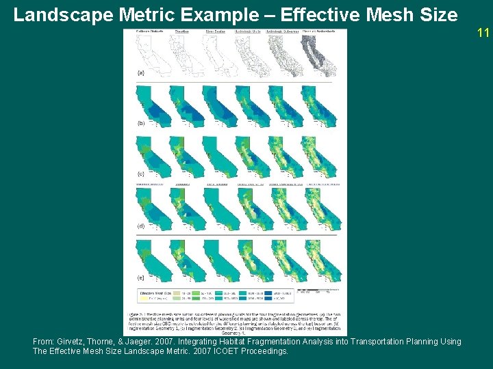
Landscape Metric Example – Effective Mesh Size 11 From: Girvetz, Thorne, & Jaeger. 2007. Integrating Habitat Fragmentation Analysis into Transportation Planning Using The Effective Mesh Size Landscape Metric. 2007 ICOET Proceedings.

Analysis Approaches 2) Graph Theory • Focused on quantifying relationships between patches • More focused on process • Solidly based in mathematical theory with many applications in other fields (e. g. geography, computer science, logistics) • Provides a language for describing relationships between patches 12

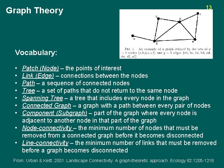
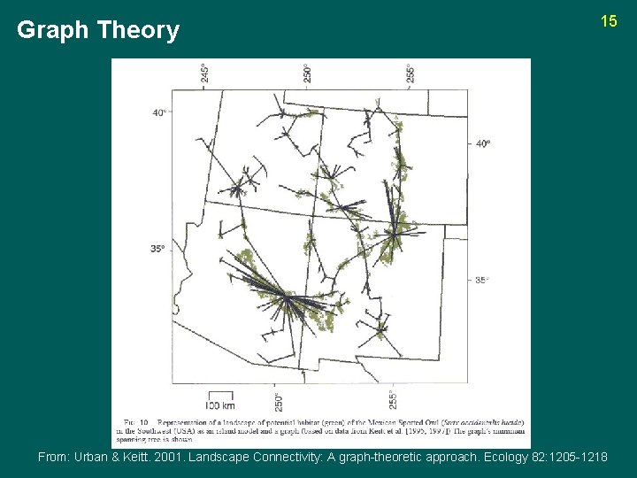
Graph Theory 13 Vocabulary: • • Patch (Node) – the points of interest Link (Edge) – connections between the nodes Path – a sequence of connected nodes Tree – a set of paths that do not return to the same node Spanning Tree – a tree that includes every node in the graph Connected Graph – a graph with a path between every pair of nodes Component (Subgraph) – part of the graph where every node is adjacent to another node in that part of the graph • Node-connectivity – the minimum number of nodes that must be removed from a connected graph before it becomes disconnected • Line-connectivity – the minimum number of links that must be removed before a graph becomes disconnected From: Urban & Keitt. 2001. Landscape Connectivity: A graph-theoretic approach. Ecology 82: 1205 -1218

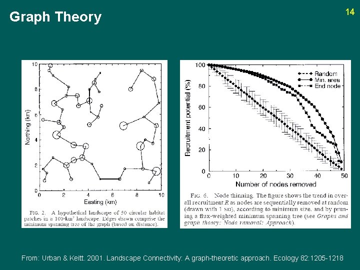
Graph Theory From: Urban & Keitt. 2001. Landscape Connectivity: A graph-theoretic approach. Ecology 82: 1205 -1218 14

Graph Theory 15 From: Urban & Keitt. 2001. Landscape Connectivity: A graph-theoretic approach. Ecology 82: 1205 -1218

Analysis Approaches 16 3) Cost-distance Analysis • More focus on matrix • Can quantify isolation between patches • Spatially explicit – can identify routes and bottlenecks • Based on the concept of “movement cost” that has some foundation in foraging theory, but lacks extensive empirical documentation • Several important assumptions about parameters and scale must be considered

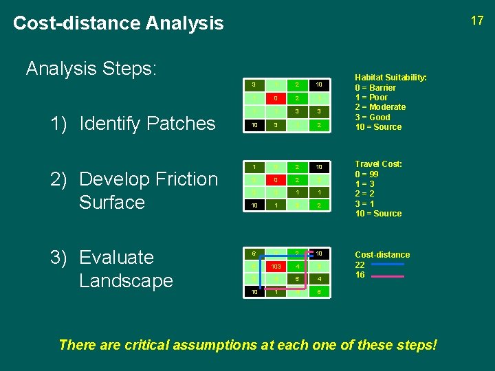
Cost-distance Analysis 17 Analysis Steps: 1) Identify Patches 2) Develop Friction Surface 3) Evaluate Landscape 3 1 2 10 1 0 2 1 1 1 3 3 10 3 1 2 1 3 2 10 3 0 2 3 3 3 1 1 10 1 3 2 6 5 2 10 6 103 4 3 3 4 5 4 10 1 4 6 Habitat Suitability: 0 = Barrier 1 = Poor 2 = Moderate 3 = Good 10 = Source Travel Cost: 0 = 99 1=3 2=2 3=1 10 = Source Cost-distance 22 16 There are critical assumptions at each one of these steps!

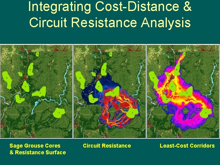
Cost-distance Analysis Results from cost-distance analysis: • Minimum cost-distance • Cost / Euclidean ratios • nth best corridor area delineations • Spatially explicit maps Many cost-distance applications have failed to take advantage of this information by focusing on least-cost paths or corridors (“Failing to see the landscape for the corridor”) 18

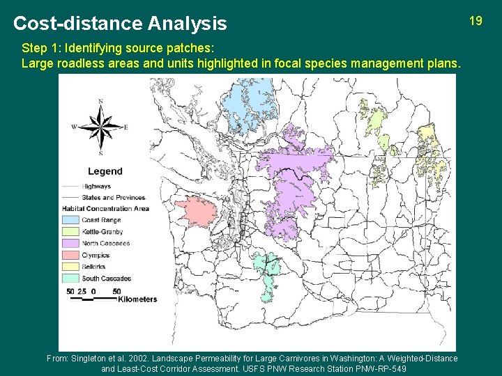
Cost-distance Analysis Step 1: Identifying source patches: Large roadless areas and units highlighted in focal species management plans. From: Singleton et al. 2002. Landscape Permeability for Large Carnivores in Washington: A Weighted-Distance and Least-Cost Corridor Assessment. USFS PNW Research Station PNW-RP-549 19

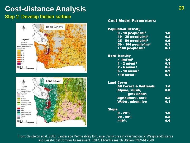
Cost-distance Analysis Step 2: Develop friction surface Road Density Land Cover 20 Cost Model Parameters: Population Density 0 - 10 people/mi 2 10 - 25 people/mi 2 25 - 50 people/mi 2 50 - 100 people/mi 2 >100 people/mi 2 1. 0 0. 8 0. 5 0. 3 0. 1 Road Density < 1 mi/mi 2 1 - 2 mi/mi 2 2 - 6 mi/mi 2 6 - 10 mi/mi 2 >10 mi/mi 2 1. 0 0. 8 0. 5 0. 2 0. 1 Land Cover All Forest & Wetlands Alpine, shrub, grasslands Agriculture, bare Water, urban, ice Slope 0 - 20% 20 - 40% >40% 1. 0 0. 8 0. 3 0. 1 1. 0 0. 8 0. 6 From: Singleton et al. 2002. Landscape Permeability for Large Carnivores in Washington: A Weighted-Distance and Least-Cost Corridor Assessment. USFS PNW Research Station PNW-RP-549

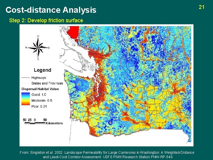
Cost-distance Analysis Step 2: Develop friction surface From: Singleton et al. 2002. Landscape Permeability for Large Carnivores in Washington: A Weighted-Distance and Least-Cost Corridor Assessment. USFS PNW Research Station PNW-RP-549 21

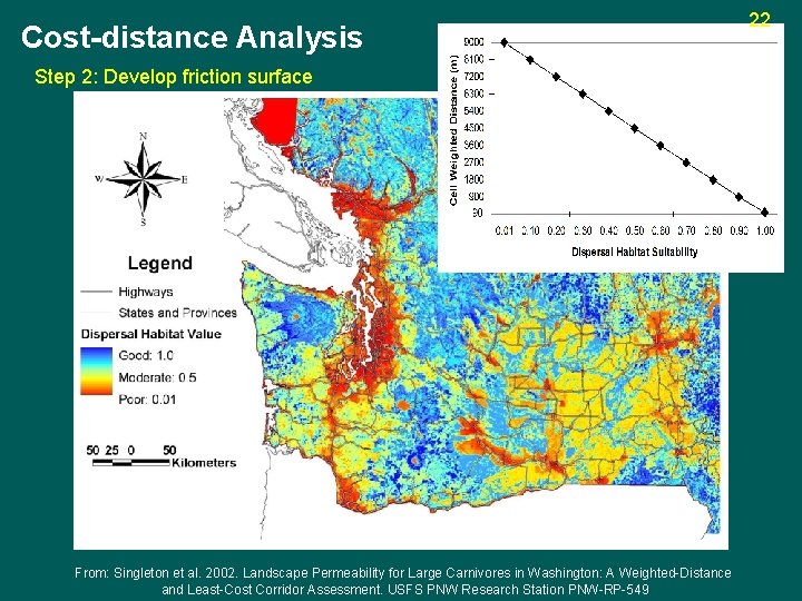
Cost-distance Analysis Step 2: Develop friction surface From: Singleton et al. 2002. Landscape Permeability for Large Carnivores in Washington: A Weighted-Distance and Least-Cost Corridor Assessment. USFS PNW Research Station PNW-RP-549 22

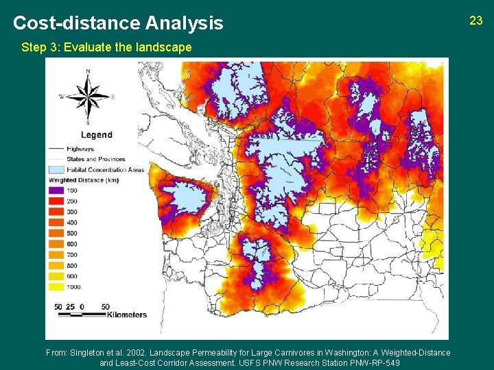
Cost-distance Analysis Step 3: Evaluate the landscape From: Singleton et al. 2002. Landscape Permeability for Large Carnivores in Washington: A Weighted-Distance and Least-Cost Corridor Assessment. USFS PNW Research Station PNW-RP-549 23

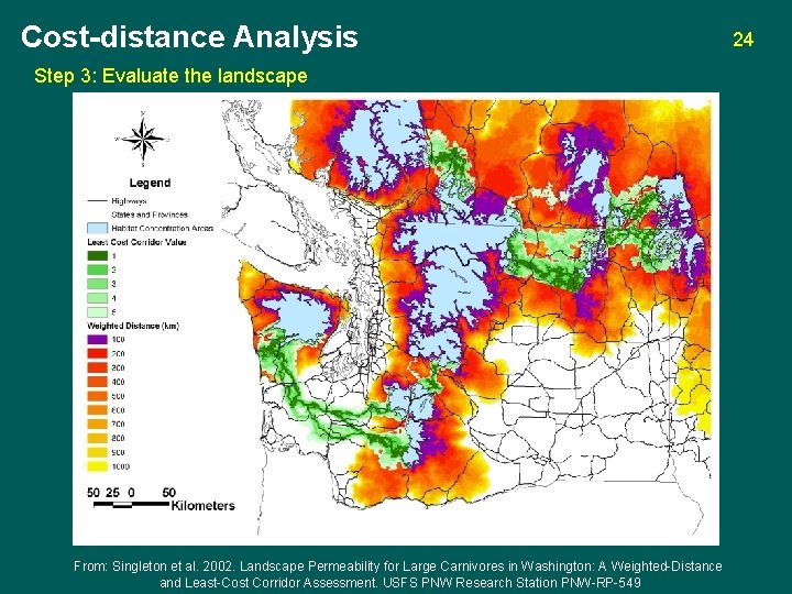
Cost-distance Analysis Step 3: Evaluate the landscape From: Singleton et al. 2002. Landscape Permeability for Large Carnivores in Washington: A Weighted-Distance and Least-Cost Corridor Assessment. USFS PNW Research Station PNW-RP-549 24

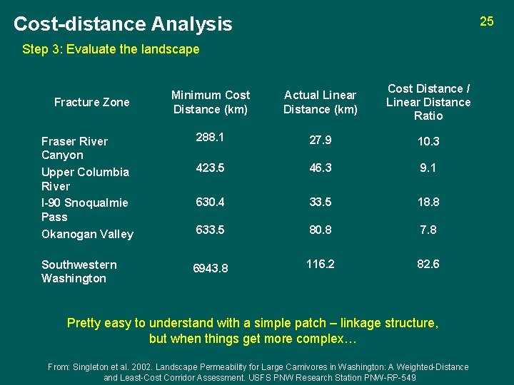
Cost-distance Analysis 25 Step 3: Evaluate the landscape Minimum Cost Distance (km) Actual Linear Distance (km) Cost Distance / Linear Distance Ratio Fraser River Canyon Upper Columbia River I-90 Snoqualmie Pass Okanogan Valley 288. 1 27. 9 10. 3 423. 5 46. 3 9. 1 630. 4 33. 5 18. 8 633. 5 80. 8 7. 8 Southwestern Washington 6943. 8 116. 2 82. 6 Fracture Zone Pretty easy to understand with a simple patch – linkage structure, but when things get more complex… From: Singleton et al. 2002. Landscape Permeability for Large Carnivores in Washington: A Weighted-Distance and Least-Cost Corridor Assessment. USFS PNW Research Station PNW-RP-549

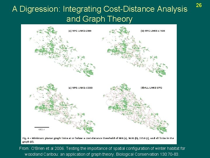
A Digression: Integrating Cost-Distance Analysis and Graph Theory From: O’Brien et al 2006. Testing the importance of spatial configuration of winter habitat for woodland Caribou: an application of graph theory. Biological Conservation 130: 70 -83. 26

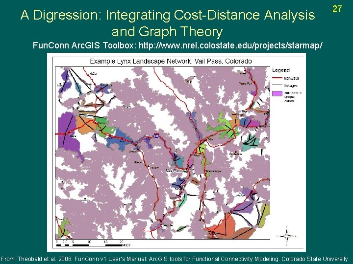
A Digression: Integrating Cost-Distance Analysis and Graph Theory 27 Fun. Conn Arc. GIS Toolbox: http: //www. nrel. colostate. edu/projects/starmap/ From: Theobald et al. 2006. Fun. Conn v 1 User’s Manual: Arc. GIS tools for Functional Connectivity Modeling. Colorado State University.

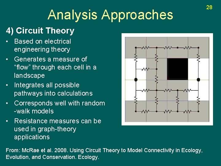
Analysis Approaches 4) Circuit Theory • Based on electrical engineering theory • Generates a measure of “flow” through each cell in a landscape • Integrates all possible pathways into calculations • Corresponds well with random -walk models • Resistance measures can be used in graph-theory applications From: Mc. Rae et al. 2008. Using Circuit Theory to Model Connectivity in Ecology, Evolution, and Conservation. Ecology. 28

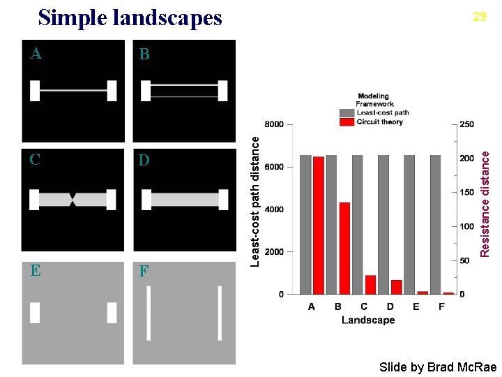
Simple landscapes C D E F Resistance distance B Least-cost path distance A 29 Slide by Brad Mc. Rae

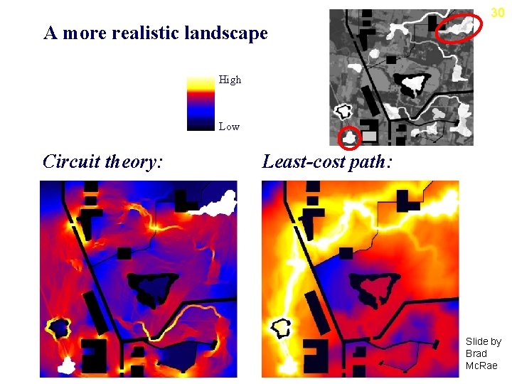
30 A more realistic landscape High Low Circuit theory: Least-cost path: Slide by Brad Mc. Rae

Integrating Cost-Distance & Circuit Resistance Analysis Sage Grouse Cores & Resistance Surface Circuit Resistance Least-Cost Corridors

Analysis Approaches 31 5) Individual Based Models & Other Approaches • Individual-based movement models (IBM) – Simulates movement of an individual through the landscape (e. g. PATH) – Many scales, from dispersal (coarse) to foraging (fine) • Population viability models (PVA) – Uses demographic information to project population persistence (covered in another chapter) • Spatially explicit population models (SEPMs) – Integrates PVA with a heterogeneous landscape where vital rates vary (e. g. Ramas GIS)

Individual-based model example: Hex. Sim 32 Hex. Sim: • IBM & SEPM • Flexible cell and group resolution • Survival / reproduction / dispersal probabilities are related to the habitat characteristics of the cell • Models individual dispersal movements through the landscape • Flexible assumptions about behavior (originally developed for spotted owl PVA, but is being applied to a variety of species) • Developed by Nathan Schumacher, EPA, Corvallis OR (http: //www. epa. gov/hexsim/)

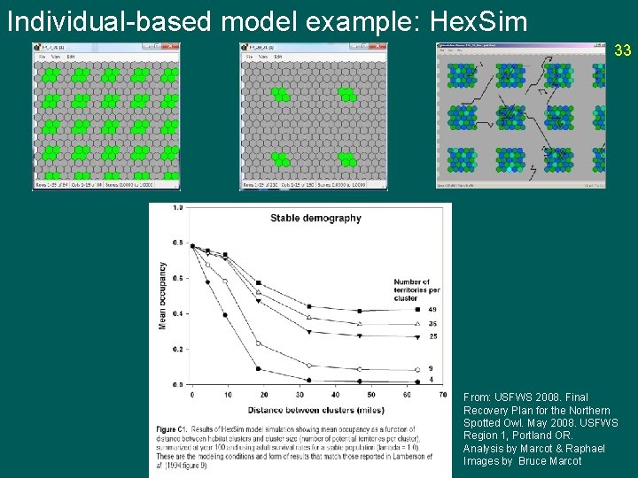
Individual-based model example: Hex. Sim 33 From: USFWS 2008. Final Recovery Plan for the Northern Spotted Owl. May 2008. USFWS Region 1, Portland OR. Analysis by Marcot & Raphael Images by Bruce Marcot

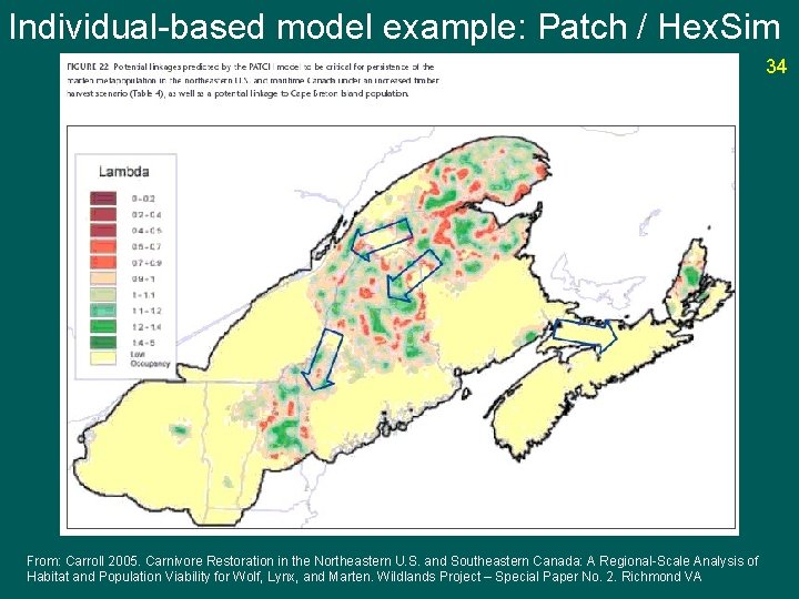
Individual-based model example: Patch / Hex. Sim 34 From: Carroll 2005. Carnivore Restoration in the Northeastern U. S. and Southeastern Canada: A Regional-Scale Analysis of Habitat and Population Viability for Wolf, Lynx, and Marten. Wildlands Project – Special Paper No. 2. Richmond VA

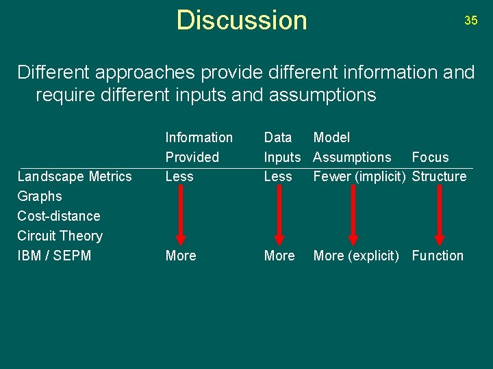
Discussion 35 Different approaches provide different information and require different inputs and assumptions Landscape Metrics Graphs Cost-distance Circuit Theory IBM / SEPM Information Provided Less Data Model Inputs Assumptions Focus Less Fewer (implicit) Structure More (explicit) Function

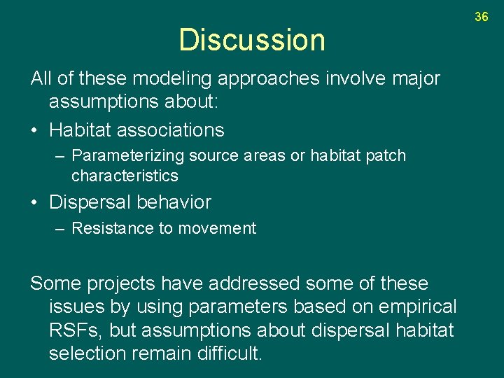
Discussion All of these modeling approaches involve major assumptions about: • Habitat associations – Parameterizing source areas or habitat patch characteristics • Dispersal behavior – Resistance to movement Some projects have addressed some of these issues by using parameters based on empirical RSFs, but assumptions about dispersal habitat selection remain difficult. 36

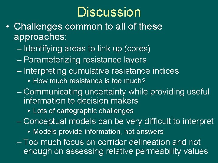
Discussion • Challenges common to all of these approaches: – Identifying areas to link up (cores) – Parameterizing resistance layers – Interpreting cumulative resistance indices • How much resistance is too much? – Communicating uncertainty while providing useful information to decision makers • Lots of cartographic challenges – Conceptual models can be very difficult to interpret • Models provide information, not answers – Too much focus on corridor delineation and not enough on assessing relative permeability values

Discussion The future of linkage modeling • Better empirical techniques: – Integration of detection probability and movement probabilty into resource selection analysis • Model validation: – Landscape genetics – GPS telemetry studies • Simulation Modeling – Hex. Sim, CDPOP • Climate Change – How do we integrate climate change concerns into connnectivity analysis? 37

Closing Pete’s cornball philosophy of landscape modeling: • Know your question • Know your data • Keep it simple • Own your assumptions • Be open to surprises, but always check twice • All models are wrong, but some models are useful • Models provide information, not answers • Validate, validate … 38