Land Use and Land Cover Chapter 20 Introduction

Land Use and Land Cover Chapter 20

Introduction l l Land use – defined by economic terms Land cover – visible features Both are important and are really inseparable We depend on accurate LU/LC data for scientific and administrative purposes

Intro l What are some examples of why knowledge of LU/LC is important?

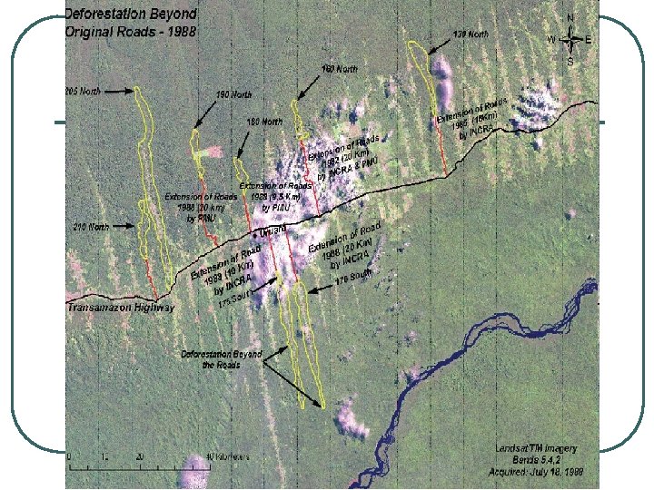
Predictive Land Use Modeling l A Basin-Scale Econometric Model for Projecting Future Amazonian Landscapes was developed to predict forest loss associated with development scenarios in the Amazon basin. • Given the scenarios, projections follow from results of econometric modeling based on economic theory and detailed local observation (led by Alexander Pfaff of Columbia University).

l As an example, this image shows a situation in which deforestation precedes road-building. • • l It depicts in red several settlement roads in 1988; deforested areas, as of 1988, are shown by the yellow polygons extending beyond the roads. Since the roads now pass through these old deforested areas, the figure suggests reverse causality, in which deforestation actually leads to road-building. • This situation is probably common in areas of smallholder colonization.

Air Photos l Most LU/LC data are derived from air photos • Used as early as 1930 by the TVA l USGS later developed a classification system

USGS Classification System l A Land Use And Land Cover Classification System For Use With Remote Sensor Data • • • By JAMES R. ANDERSON, ERNEST E. HARDY, JOHN T. ROACH, and RICHARD E. WITMER Geological Survey Professional Paper 964 A revision of the land use classification system as presented in U. S. Geological Survey Circular 671

Classification Level Typical data characteristics I LANDSAT (formerly ERTS) type of data II High-altitude data at 40, 000 ft (12, 400 m) or above (less than l: 8 O, OOO scale) III Medium-altitude data taken between 10, 000 and 40, 000 ft (3, 100 and 12, 400 m) (1: 20, 000 to 1: 80, 000 scale) IV Low-altitude data taken below 10, 000 ft (3, 100 m) (more than 1: 20, 000 scale)

Level II 1 Urban or Built-up Land 11 Residential 12 Commercial and Services 13 Industrial 14 Transportation, Communications, and Utilities 15 Industrial and Commercial Complexes 16 Mixed Urban or Built-up Land 17 Other Urban or Built-up Land

2 Agricultural Land 21 Cropland Pasture 22 Orchards, Groves, Vineyards, Nurseries, and Ornamental Horticultural Areas 23 Confined Feeding Operations 24 Other Agricultural Land

3 Rangeland 31 Herbaceous Rangeland 32 Shrub and Brush Rangeland 33 Mixed Rangeland 4 Forest Land 41 Deciduous Forest Land 42 Evergreen Forest Land 43 Mixed Forest Land

Visual Interpretation l Interpreters look at imagery and draw boundaries to mark categories • Use the numeric symbols of the classification system l Remember chapter 5 about visual interpretation cues

Visual Interpretation l Cropped agricultural land is recognized by systematic division of fields into rectangles or circles, with smooth even textures. • Tone varies with growth stage l Pasture is usually more irregular in shape, a mottled texture, medium tone with possibly some isolated patches of trees

Visual Interpretation l Transportation is often seen as linear patterns that cut across the landscape, and by distinctive loops of interchanges

Visual Interpretation l Some parcels are delineated as multiple purpose • Airports – include runways, hangars, terminals, roads, etc.

Land Use Change by Visual Interpretation l Two maps representing the same region are prepared for different dates, to depict land use/land cover • Must use the same classification system • One can’t be “forest” if the other splits into “pine” and “deciduous” • Must be compatible with respect to scale, geometry, and level of detail • Should be able to identify points on both maps

Historical and Environmental Analysis l Aerial photos are helpful where hazardous materials may have been used/abandoned • Disposal sites include ponds, lagoons, • landfills, etc. These may now be in populated areas due to urban sprawl

Other LU/LC classification systems l The Anderson system described earlier is a general-purpose classification system • Land Utilization Survey of Britain • TVA land use • New York Land Use and Natural Resources Survey

Other LU/LC classification systems l Special Purpose Classification Systems • Wetlands Classification (Cowardin, 1979)

Land-Cover Mapping by Image Classification l Appears straightforward, but many factors are hidden • Selection of images – what season, what • dates are of most significance Processing – accurate registration and atmospheric corrections • Subsetting needs to be done carefully • Classification algorithm – needs to be chosen based on region • “grow” homogenous training fields

Land-Cover Mapping by Image Classification l l Assignment of spectral classes to informational classes – “deciduous forest” may require spectral classes that reflect slope aspect. Display and symbolization – consistency of color choices

Digital Compilation of Land-Use l Probably no one set of techniques works in all situations. Digital change (Jensen 1996) • Image algebra – image subtraction where values near zero are no change, usually applied to single band • Must select threshold for change/no change • Image ratios can also be applied

Digital Compilation of Land-Use • Postclassification comparisons – independent classification of scenes which are then compared • Accurate classification is required • Multidate composites – assemble all bands from multiple dates into a single composite. The entire set is then analyzed by principle components or other techniques • Pretty unwieldy

Digital Compilation of Land-Use • • Spectral change vector analysis – examines a pixel’s position in multispectral data space. If the pixel occupies roughly the same position in the two data sets, it has not changed. Binary change mask – classify first date, do image algebra on original images from both dates, create a binary mask representing only changed/unchanged pixels. Classify the second date, but use only the pixels identified as changed in the mask.

Digital Compilation of Land-Use • On-screen digitization – software is used to • view both images side-by-side and visually interpret them. Change detection by image display – corresponding bands from different dates are used as separate overlays in RGB display

Broad-scale Land-Cover studies l l AVHRR and other data has been used to look at continental or hemispheric changes over time LULC Multiresolution Land Characteristics Gap Analysis