Lamports Scalar Clocks Shiva Bottu Organization Introduction High

Lamport’s Scalar Clocks Shiva Bottu

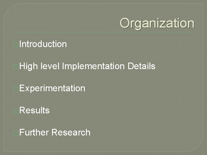
Organization �Introduction �High level Implementation Details �Experimentation �Results �Further Research

Introduction � Lamport’s logical clocks are introduced to capture causality relation in a distributed system. � Each process Pi has a logical clock Ci and for a particular event a in P, it assigns an integer value Ci, which is timestamp of the event. � Timestamps are monotonically increasing.

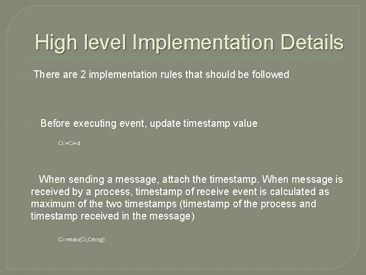
High level Implementation Details � 1. There are 2 implementation rules that should be followed Before executing event, update timestamp value Ci: =Ci+d 2. When sending a message, attach the timestamp. When message is received by a process, timestamp of receive event is calculated as maximum of the two timestamps (timestamp of the process and timestamp received in the message) Ci: =max(Ci, Cmsg)

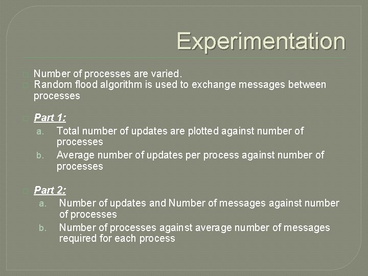
Experimentation � � Number of processes are varied. Random flood algorithm is used to exchange messages between processes � Part 1: a. Total number of updates are plotted against number of processes b. Average number of updates per process against number of processes � Part 2: a. Number of updates and Number of messages against number of processes b. Number of processes against average number of messages required for each process

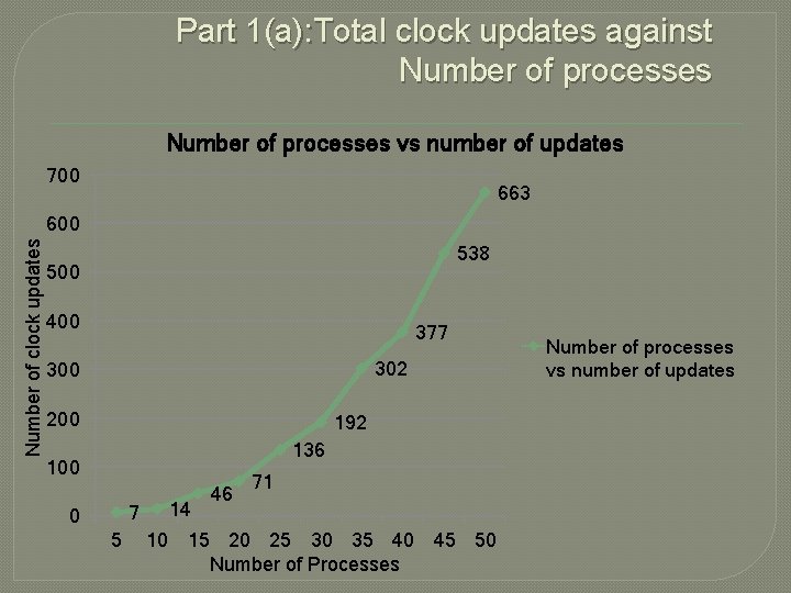
Part 1(a): Total clock updates against Number of processes vs number of updates 700 663 Number of clock updates 600 538 500 400 377 302 300 200 192 136 100 7 0 5 14 46 71 10 15 20 25 30 35 40 45 50 Number of Processes Number of processes vs number of updates

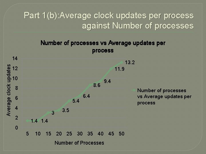
Part 1(b): Average clock updates per process against Number of processes vs Average updates per process Average clock updates 14 13. 2 12 11. 9 10 8. 6 8 6 5. 4 4 3 2 9. 4 6. 4 3. 5 1. 4 0 5 10 15 20 25 30 35 40 45 50 Number of Processes Number of processes vs Average updates per process

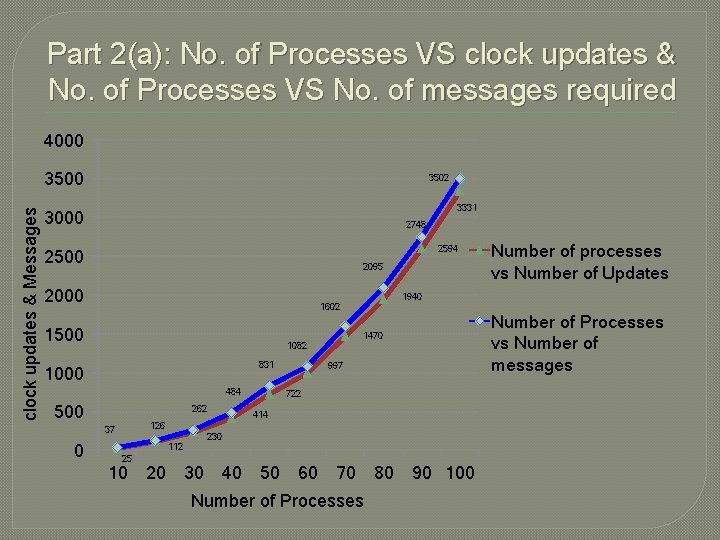
Part 2(a): No. of Processes VS clock updates & No. of Processes VS No. of messages required 4000 clock updates & Messages 3500 3502 3331 3000 2748 2594 2500 2095 2000 1940 1602 1500 831 484 500 262 Number of Processes vs Number of messages 1470 1082 1000 997 722 414 126 37 0 Number of processes vs Number of Updates 230 112 25 10 20 30 40 50 60 70 Number of Processes 80 90 100

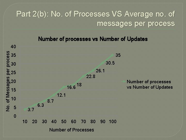
Part 2(b): No. of Processes VS Average no. of messages per process Number of processes vs Number of Updates No. of Messages per process 40 35 35 30 26. 1 25 22. 8 20 16. 6 15 12. 1 10 5 18 3. 7 6. 3 8. 7 0 10 20 30 40 50 60 70 80 90 100 Number of Processes Number of processes vs Number of Updates

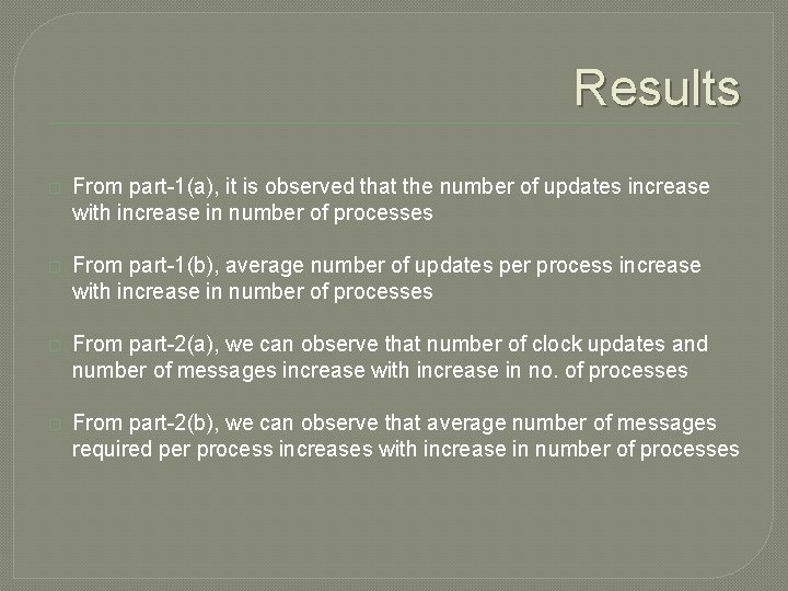
Results � From part-1(a), it is observed that the number of updates increase with increase in number of processes � From part-1(b), average number of updates per process increase with increase in number of processes � From part-2(a), we can observe that number of clock updates and number of messages increase with increase in no. of processes � From part-2(b), we can observe that average number of messages required per process increases with increase in number of processes

Further Research � To change the base algorithm from random flood to other topologies and test with the same process. � Running with high load of processes.

References �http: //en. wikipedia. org/wiki/Lamport_timest amps �http: //cnlab. kaist. ac. kr/~ikjun/data/Course_ work/CS 642 Distributed_Systems/papers/lamport 1978. pdf