Lagrangian models Lagrangian particle models are threedimensional models

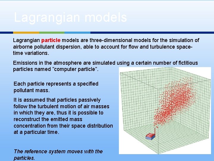
Lagrangian models Lagrangian particle models are three-dimensional models for the simulation of airborne pollutant dispersion, able to account for flow and turbulence spacetime variations. Emissions in the atmosphere are simulated using a certain number of fictitious particles named ”computer particle”. Each particle represents a specified pollutant mass. It is assumed that particles passively follow the turbulent motion of air masses in which they are, thus it is possible to reconstruct the emitted mass concentration from their space distribution at a particular time. The reference system moves with the particles.

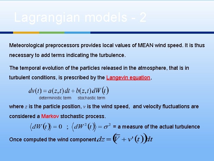
Lagrangian models - 2 Meteorological preprocessors provides local values of MEAN wind speed. It is thus necessary to add terms indicating the turbulence. The temporal evolution of the particles released in the atmosphere, that is in turbulent conditions, is prescribed by the Langevin equation, deterministic term stochastic term where z is the particle position, v is the wind speed, and velocity fluctuations are considered a Markov stochastic process. = a measure of the actual turbulence Once computed the wind component,

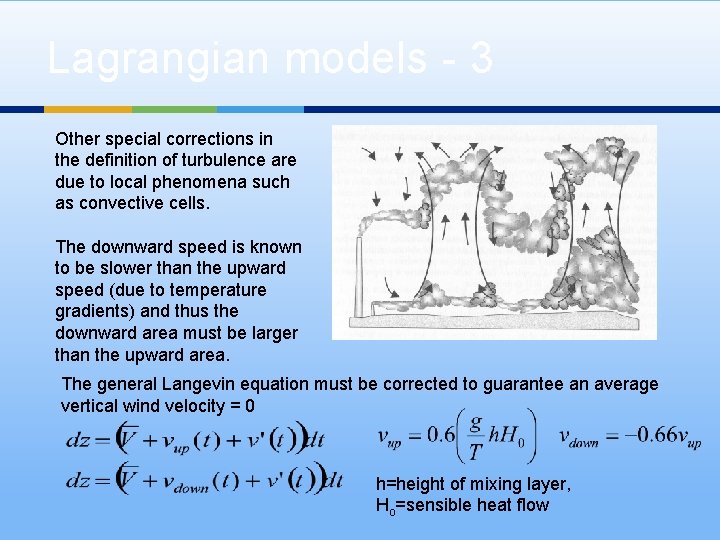
Lagrangian models - 3 Other special corrections in the definition of turbulence are due to local phenomena such as convective cells. The downward speed is known to be slower than the upward speed (due to temperature gradients) and thus the downward area must be larger than the upward area. The general Langevin equation must be corrected to guarantee an average vertical wind velocity = 0 h=height of mixing layer, Ho=sensible heat flow

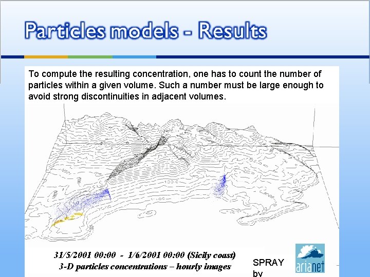
Particles models - Results To compute the resulting concentration, one has to count the number of particles within a given volume. Such a number must be large enough to avoid strong discontinuities in adjacent volumes. 31/5/2001 00: 00 - 1/6/2001 00: 00 (Sicily coast) 3 -D particles concentrations – hourly images SPRAY by

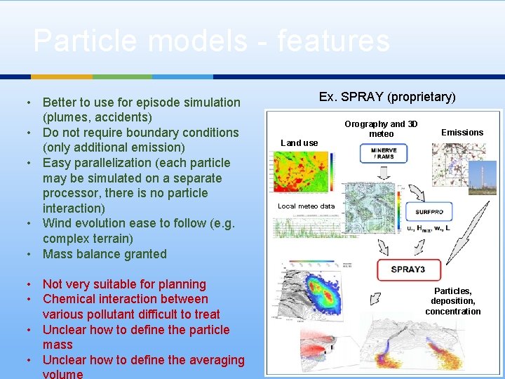
Particle models - features • Better to use for episode simulation (plumes, accidents) • Do not require boundary conditions (only additional emission) • Easy parallelization (each particle may be simulated on a separate processor, there is no particle interaction) • Wind evolution ease to follow (e. g. complex terrain) • Mass balance granted • Not very suitable for planning • Chemical interaction between various pollutant difficult to treat • Unclear how to define the particle mass • Unclear how to define the averaging Ex. SPRAY (proprietary) Land use Orography and 3 D meteo Emissions Local meteo data Particles, deposition, concentration

Trajectory models Used for long-range transport, heavy metals, acid rains (and consequent acidification and eutrophication). Similar to particle models, but the pollution “unit” is a air column with a height equal to the mixing layer. They are transported in the domain by a 3 D wind field. If s(t) is the column position at time t and V(t) is the 3 D wind field: ds(t)/dt=V(t) Assuming a coordinate system centered in the column position and moving (horizontally) with it: + chemical reactions (s(t)) + net input(s(t))

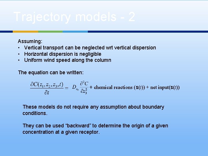
Trajectory models - 2 Assuming: • Vertical transport can be neglected wrt vertical dispersion • Horizontal dispersion is negligible • Uniform wind speed along the column The equation can be written: + chemical reactions (s(t)) + net input(s(t)) These models do not require any assumption about boundary conditions. They can be used “backward” to determine the origin of a given concentration at a given receptor.

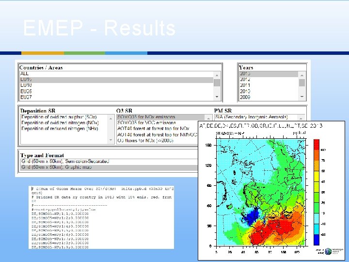
Trajectory models - EMEP It is the model developed within the Cooperative program for the monitoring and evaluation of the long-range transmission of air pollutant in Europe (mostly by the Norwegian Meteorological Institute, since 1979). Fortran code available. It formed the basis for the Gothenburg Protocol negotiations (transboundary pollutants) signed in 1999. Its resolution is 50 x 50 km 2 and mainly considered emissions of NOx, SO 2, NH 3 to compute the corresponding concentrations of 10 different species, including for instance PANs (Peroxyacyl) that are powerful respiratory and eye irritants present in photochemical smog. From a number of simulations, it has been derived an IMPACT MATRIX (a linear surrogate model) that shows the effect of the emissions of each 50 x 50 km 2 grid in Europe on all the other 50 x 50 km 2 grids.

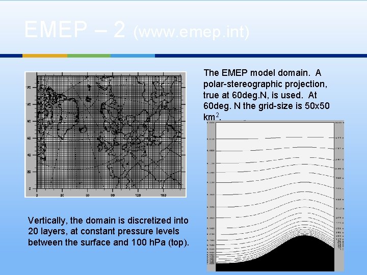
EMEP – 2 (www. emep. int) The EMEP model domain. A polar-stereographic projection, true at 60 deg. N, is used. At 60 deg. N the grid-size is 50 x 50 km 2. Vertically, the domain is discretized into 20 layers, at constant pressure levels between the surface and 100 h. Pa (top).

EMEP - Results