Lagrangian Method Classical Mechanics By Barger and Olsson

• Different forms of Newton’s equations of motion depends on coordinates

Rectangular Components – Cartesian Coordinates or

Tangential and Normal Components y m And as a reminder O z x

EQUATIONS OF MOTION IN TERMS OF RADIAL AND TRANSVERSE COMPONENTS Consider particle at r and q, in polar coordinates, y O x

EQUATIONS OF MOTION IN TERMS OF SPHERICAL COORDINATES

• The Lagrangian method makes it simple to write the equations of motion in any coordinate system. • It makes it simpler to work with constraints and to identify conserved quantities. • The Lagrangian method makes it easier to find the equations of motions for certain problems. • Lagrange’s equations and the related Hamilton’s equations are of fundamental importance to classical mechanics and quantum mechanics.

Lagrange Equation • • Consider a system of N particles in three dimensional space. There are 3 N cartesian coordinates needed to describe their motions. There is a Newton’s equation for each of these coordinates. A first step to the Lagrange method is to choose a new set of coordinates called general coordinates. • • (3. 1)

• The set of {qj} collectively describe the configuration of the system. • These coordinates are not necessarily of distance dimensions. Often they are angles. • Example of one particle in spherical polar coordinates (r, q, f). (3. 2)

• If particle moves on the surface of a sphere of radius l centered at the origin, then only q and f vary in time. • A relation of this type is called a constraint. • Equations of motion which result directly from the substitutions of (3. 1) in Newton’s equations are usually messy. • Lagrange’s equations are much nicer. They show explicitly the simplifications of symmetries and constraints. • Lagrange equations are not the same as Newton ‘s but are equivalent. • In fact each Lagrange equation is a linear combination of Newton’s equations, and vice versa.

Lagrange’s Equations in One Dimension • We introduce a general coordinate q(t) expressed in terms of x by (3. 3) or (3. 4)

• Chain differentiation (3. 5) • The partials are functions of q and t. • The momentum is (3. 6)

• Introduce a new momentum p(t) called the generalized momentum • • Where • From (3. 4) and (3. 5) (3. 7) (3. 8) (3. 9)

• Therefore (3. 10) • Newton’s equation of motion. (3. 11) • The corresponding Lagranian equation of motion involves the time derivative of p. Take the derivative of both sides of 3. 10.

(3. 12) • To simplify the second term we interchange the order of differentiation. (3. 13)

• We digress to show 3. 13 (3. 14) • In Lagrangian formalism q and are independent variables in the sense that

• Differentiating 3. 5 (3. 15) • Since the right-hand sides of 3. 14 and 3. 15 are identical, then 3. 13 follows. (3. 14) (3. 13)

• Multiple 3. 13 times p and replace p on right-hand side with 3. 6. (3. 13) (3. 6) (3. 16)

Substitute 3. 11 and 3. 16 into 3. 12 (3. 11) (3. 16) (3. 12) (3. 17)

(3. 17) The first term on the right-hand side is called the general force (3. 18) Then the equation of motion (3. 19) The last term in this equation represents a “fictitious” force which appears whenever the coefficients in 3. 5 vary with q.

If the force F is separated into a part and a part that is not, then the general force can be separated into corresponding parts. (3. 20)

3. 20 into 3. 19 (3. 21) Where (3. 22) This is the Lagrangian function.

• Since (3. 23) • follows from 3. 7 and

Then 3. 21 can be written (3. 24) The general force for Q’ must include all forces F’ on the particle which are not included in the potential energy.

Lagrange’s Equations in Several Dimensions • For 3 D follow previous procedure, step by step • There are now 3 N cartesian components and likewise 3 N general coordinates • In analogy to (3. 6) we have (3. 24) (3. 25) (3. 26)

• In parallel to the derivation in one dimension we find (see (3. 17 and 3. 18)) (3. 27)

• Where L is the Lagrangian (3. 28) The general forces derived from a potential are (see (3. 18)) (3. 29)

• and (3. 30) • are the other general forces. It follows from (3. 25) and that the general momentum can be written as (3. 31)

• So (3. 27) becomes (3. 32)

Elementary application of Lagrangian techniques Determine the r and q equations of motion for a particle moving in a plane under the influence of a central potential energy V(r). As general coordinates we take (3. 33) (3. 34) (3. 35)

• Easy to express in polar coordinates by taking time derivatives. (3. 36) (3. 37) • Note that K is not a function of q 2.

• The Lagrangian is (also see (3. 32)) (3. 38) (3. 39) (3. 40)

• The previous were obtained from direct application of Newton’s laws with • Since L does not depend on q , (3. 27) • hence the general momentum is constant, (3. 41)

• This conservation law is an example of a general principle that can be deduced from the Lagrange equation. If a general coordinate does not appear in the Lagrangian and • The corresponding general momentum • is constant in time. It is a constant of the motion (a conserved quantity).

Constraints • Example of constrained motion – the simple pendulum • The tension will be the constraint force. • Note that the number of unknown components of constraint force must be the same as the number of constraints on the motion, otherwise the motion will be over- or under-determined. (This refers to more equations or less equations than the number of unknowns. )

• How can we systematically treat a mechanical system with constraints? The first step is to find combinations of the Newton equations in which the constraint forces are absent. As we shall moreor-less demonstrate below, these are precisely Lagrange equations, for an appropriate choice of coordinates. One has enough information to solve these equations (while assuming the constraints to hold), and the solutions to these determine the motion. The remaining equations, into which one substitutes the solution to the motion, then determine the constraint forces; if only the solution for the motion were desired, this step would be unnecessary.

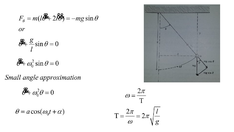
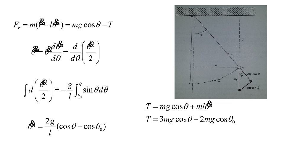
Now using Lagrangian Method Lagrangian in polar coordinates, with r = l

Radial Lagrangian equation

The constraint force is the negative of the tension.

Angular Lagrangian equation

• The result of the above exercise is that: • 1. We can impose constraints directly in the Lagrangian and determine the correct equations of motion without ever explicitly referring to the constraint forces. • 2. If we wish to find the force required to enforce a constraint, we choose an additional general coordinate (in this case r) so that when it is held to a particular constant (r = l here) the constraint is maintained. The constraint force then follows as in (3. 46).

Hamiltonian Dynamics* • If the potential energy of a system is velocity independent, then the linear momentum components in rectangular coordinates are given by • In general coordinates * Classical Dynamics by Marion and Thornton

• The Hamiltonian may be written as The Lagrangian is considered to be a function of the generalized coordinates, the generalized velocities, and possibly the time. The dependence of L on the time may arise either if the constraints are time dependent or if the transformation equations connecting the rectangular and generalized coordinates explicitly contain the time. The Hamiltonian is always considered as a function of the

• H is the total energy if the following conditions are met. • The equations of the transformation connecting the rectangular and generalized coordinates must be independent of the time. • The potential energy must be velocity independent. • The equations of motion are

• Using the Hamiltonian method, find the equations of motion for a spherical pendulum of mass m and length b. • The generalized coordinates are q and f. b q f • The generalized momenta are then

b q f

• The equations of motion are b q f

• The equations of motion are b q f • Because f is cyclic, the momentum about the symmetry axis is constant.