Labour supply Readings Borjas ch 2 not 2
 Labour Force")
Labour supply Readings: Borjas, ch. 2 (not 2. 13 and 2. 14) Labour Force Surveys (Current Population Surveys in US): The labour market at a given moment – shows stocks. Stock: – for example, the number of people who are unemployed at some point in time. Flow: For example the numbers who enter or leave unemployment during a period of time. We want to know: ◦ How long are people unemployed? ◦ Have they quit, been fired or are they new entrants? ◦ WHAT HAPPENS TO THEM?

Flows on the labour market The labour market as a dynamic system: Arrows = labour market transitions Not in labour force Employed Unemployed Ex: Unemployment Sweden 2002: 176 400 Flow into unemployment = 525 000 75 % previously employed, 25 % new entrants or re-entering

Labour market survey. Sweden 2010 Population in age span 15 -74 years. in thousands Population 7 022 In the labour force 4 962 Employed 4 546 At work 3 869 Of which underemployed 316 Outside the labour force 2 060 Wanted to work Unemployed 416 (of which 127 full-time students) Absent week of survey 678 Could have taken a job 129 (latent unempl. ) Did not want to work Would have wanted but could not have taken job

Not in labour force 2 060 Ill 376 Full time students 569 Retired 837 Others 278 Absent 678 Illness 89 Vacation 383 Parental leave 114 Other reason 92

Definitions in labour market statistics: Labour force surveys – surveys of a probability sample of the population. Usually monthly. Refer to one week. In the labour force (economically active) = employed or unemployed Employed = worked for pay or profit at least one hour or unpaid in family farm/business or was on leave (vacation. sick-leave. parental leave etc. ) Unemployed – wanted to work; was able to take up a job if offered and actively searched for a job in the last four weeks. (In Sweden. until 2005 full -time students could not be counted as unemployed. )

At work – employed and worked at least one hour during the reference week. Latent unemployed (discouraged) – was able to and wanted to work but did not actively search Another category wanted to work but would not have been able to take a job (disability. lack of child-care facilities etc. ) If nothing else is specified, all statistics in these notes are from the LFS of Statistics Sweden.

Female and male participation rates at age 16 -64, Sweden 1976 -2009 1 0. 9 0. 8 0. 7 0. 6 0. 5 Women 0. 4 Men Women 0. 3 Men 0. 2 0. 1 19 19 76 78 19 80 19 82 19 84 19 86 19 88 19 90 19 92 19 94 19 96 19 98 20 00 20 02 20 04 20 06 20 08 0 Note the change of definition in 2005

Participation 1976 and 2004 1. 2 Participation rate 1 0. 8 Men 1976 Men 2004 0. 6 Women 1976 Women 2004 0. 2 0 16 -19 20 -24 25 -34 35 -44 Age 45 -54 55 -59 60 -64

90 80 Participation rates according to education 70 60 50 Women 40 Men 30 20 10 0 primary secondary post-secondary Age 16 -74 Source: Statistics Sweden

Labour supply over 40 years in Sweden: • • In 1965 the average number of hours worked per capita (aged 16 -64) was 26. 8. 25 years later it was 26. 2. In 2003. after the deep recession of the 1990 s. it was 22. 3. But the almost constant average is made up of several components and these had changed much more.
 Employed/ Unemploy labour force -ment (%) Hours of")
Labour force/ popula tion (%) Employed/ Unemploy labour force -ment (%) Hours of At work of work per employ Hours if at capita ed % work Men 1965 89. 3 0. 8 99. 2 91. 7 45. 8 37. 2 Men 2003 79. 9 5. 3 94. 7 86. 2 38. 9 25. 4 Women 1965 53. 8 1. 8 98. 2 88. 3 35. 0 16. 3 Women 2003 76. 2 4. 4 95. 6 79. 4 33. 0 19. 1 Source : Björklund. Edin. Holmlund & Wadensjö: Arbetsmarknaden

To be employed is not the same as being at work and working full-time. Men 15 -74 2010 Women 15 -74 2010 Shares in percent Average With children 1 -2 yrs Average Participation rate 76. 1 Participation rate Unemployment Employment rate* At work rate** Work hours of those at work Part time 1 -35 hours 8. 5 67. 6 87. 4 Unemployment 8. 2 Employment rate* 61. 8 At work rate** 82. 5 Work hours of 27. 5 those at work Part time 1 -35 hours. 35. 9 * Employed/population 90. 6 33. 1 12. 8 32 **At work/employed * Employed/population work/employed With children 1 -2 yrs 70. 0 75. 6 24 **At

Participation in different countries Men 1973 Men 2003 Change Women 1973 Women 2003 Change Canada 86. 1 83. 8 -2. 3 47. 2 73 25. 8 Denmark 89. 6 84 -5. 6 61. 9 74. 8 12. 9 80 76. 1 -3. 9 63. 6 72. 1 8. 5 France 85. 2 73. 8 -11. 4 50. 1 62. 5 12. 4 Ireland 92. 3 78. 3 -14 34. 1 57. 6 23. 5 Italy 85. 1 74. 8 -10. 3 33. 7 48. 3 14. 6 Japan 90. 1 84. 6 -5. 5 54 59. 9 5. 9 Norway 86. 5 82. 9 -3. 6 50. 6 75. 9 25. 3 Spain 92. 9 81. 1 -11. 8 33. 4 55. 7 22. 3 Sweden 88. 1 80. 8 -7. 3 62. 6 76. 9 14. 3 Germany 89. 6 78 -11. 6 50. 3 64. 9 14. 6 UK 93 83. 9 -9. 1 53. 2 69. 2 16 US 86. 2 82. 2 -4 51. 1 69. 7 18. 6 All OECD 88. 2 80. 2 -8 48. 3 59. 6 11. 3 Finland

International trends in labour supply: Lower participation of young people (longer schooling, later labour market entry) Lower participation of older men (earlier retirement) Higher participation of women Decrease in difference between married and single or divorced women High female participation in Nordic countries

Why is the participation rate high for women in Sweden? Separate taxation since 1971 Publicly provided and subsidised child-care Parental leave A large public sector which employs many women High level of female education Smaller gender wage differentials than in other countries
")
Unemployment and labour force participation During recessions (e. g. Sweden in the 1990 s) participation rates fall The ”discouraged worker”-effect • some give up searching because they despair of finding a job • there are more publicly funded labour market training programs • people study although they would have preferred to work There is also an ”added worker”-effect in households

Thousands outside the labour force who wanted to and were able to work in 1990, 1994, 1998 and 2002

Summary of changes in labour supply. Sweden 19652003 Average number of hours worked per capita decreased by nearly 4½ hours Hours worked by men decreased by nearly 12 hours Hours worked by women increased. by just under 3 hours Male participation decreased by 10 percentage points Female participation increased by 20 percentage points Unemployment increased dramatically to ”Western European levels” in 1990 s. It has now fallen substantially but not back to historical levels. Absence from work up from 9. 5 to 17 percent. The increase is twice as large for women as for men. (Longer yearly holidays and parental leave. ) The average time worked among those who are at work decreased. more for men than for women.
 economic analysis of labour supply studies: ECONOMIC factors and:")
Theories of labour supply (Mainstream) economic analysis of labour supply studies: ECONOMIC factors and: - the decision to work or not to work - the decision how many hours to work Variables: Net wage (rate) & non-labour income. (Costs of working. ) The simplest model: Other factors exist but are assumed to be constant Each member of a household is treated as an isolated individual. The model is static – consequences in the future do not affect the present.

Digression on models and theories All theories are abstract – abstract from something The ”something” should either be less important or assumed to be held constant What are REASONABLE and FRUITFUL abstractions depends on what is being analysed
: Marital status and children Ethnicity")
Labour supply depends on (besides wage, income and costs): Marital status and children Ethnicity Age Gender Social class Education Norms of what is appropriate at a particular time and place for a person of a given gender, age, social class, ethnicity, education etc. THE ECONOMIC THEORY DOES NOT SAY THAT THESE ARE UNIMPORTANT – IT LOOKS AT THE EFFECT OF ECONOMIC FACTORS GIVEN THE OTHERS

This simple model which we begin with is an example of: Partial analysis – all other factors are kept constant. Individualistic – one person’s labour supply doesn’t make any difference to anyone else’s Static- the model refers to one single point in time More sophisticated models exist in empirical studies other explanatory variables are included in the model there are theoretical models of how the labour supply of household members depend on the others. This can be done in different ways: ◦ The working time of other household members is taken as given ◦ The household is seen as a unit with a joint utility function ◦ Game theoretic models or bargaining models of decision making where household members have conflicting preferences Life cycle models take into account that labour supply at one point in time has an impact and depends on labour supply over the rest of one’s life.

The basic assumptions of the model: - Each individual maximises his/her utility - Individual utility is a function of consumption of goods and services and of leisure (work has a net disutility) - The individual has a certain amount of available time which is divided between market work and leisure - Feasible consumption depends on earnings (hourly wage *time in market work) + nonlabour income - The marginal utilities of leisure and consumption are always positive (“the more the bettter”) - The marginal utilities of leisure and consumption are decreasing (indifference curves are convex to the origin).
 (1) subject to the")
The model formalised The individual maximises: U = f(C, L) (1) subject to the constraints C = h*w + V (3) L+h=T (2) Partial derivatives of U are > 0 and decreasing U L C T h w V Utility Leisure (hours) Consumption (of market goods) Total time available (24 h/day. 168 h/week. 8760 h/year) time in market work (hours) (hourly) wage rate non-labour income

Indifference curves of one individual: C L

The slope of the indifference curve shows the MARGINAL RATE of SUBSTITUTION between consumption and leisure. Example 1. Anna has 16 hours of leisure per day and a net income of 560 kronor. Her level of utliity is unchanged if she gives up ½ hour of leisure and gains 40 kronor in income. Marginal rate of substitution: If Anna had 20 hours of leisure per day and a net income of 280 kronor. she would be indifferent to working another two hours if she gets 130 kronor. Marginal rate of substitution Generally: An individual is indifferent between L 0 hours of leisure and Y 0 kronor in income OR L 1 hours of leisure and Y 1 kronor in income. She can substitute ΔY = Y 1 - Y 0 for 0 ΔL = L 1 - L 0 The marginal rate of substitution is

Different individuals have different preferences when it comes to leisure versus money. This is reflected in different indifference curves. Please note: Indifference curves of different individuals can intersect! “Red” has stronger preferences for consumption. “Blue” for leisure.

The budget constraint The slope of the orange line is equal to the hourly wage rate. w V+ WT V+W V W Non-labour income V T-1 T

Choice of optimal labour/leisure time

The optimal choice is at a point of tangency between the budget constraint and an indifference curve. It depends on the budget constraint (w and V) AND on preferences. Tangency the slope of the budget constraint = the slope of the indifference curve At the optimum. marginal utilities are proportionate to prices.

Labour supply of individuals with different preferences:

Non-labour income and labour supply Increase in non-labour income decrease in labour supply if leisure is a normal good V 2 V 1 L 2

A change in the wage rate has TWO effects on labour supply The substitution effect: "The commodity leisure" gets more expensive relative to markets goods for consumption. “The cost of not working” increases. All else equal. labour supply should increase. The income effect: With a higher wage the value of the ”endowment of time” increases. With an increase in wealth one can afford to work less. It is possible to work less and earn as much or more. All else equal. labour supply should decrease. The two effects tend in opposite directions. Theory cannot predict which effect will dominate – whether a wage increase leads to increase or decrease in labour supply is an empirical question.
 Consumption ($)")
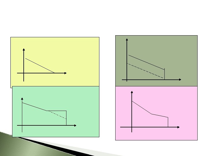
More leisure at higher wage When the Income Effect dominates (equivalent variation) Consumption ($) G U 1 R D Q U 0 F D P V E 0 70 75 85 110 Hours of Leisure
. Consumption")
More work at a higher wage When the Substitution Effect dominates (equivalent variation). Consumption ($) U 1 G R D Q U 0 F D P V E 0 65 70 80 110 Hours of Leisure

Another measure – the compensating variation An example where the substitution effect dominates: Blue line = original budget line Red line = budget line after wage increase Dotted green line = (imaginary) allows the consumer to just reach the same level of utility as before the wage increase

Reservation wage Wr: If W < Wr The individual will not work If W > Wr The individual will work If W = Wr The individual will be indifferent between working and not working

The red full line represents a wage at which the individual will be best off if she works. The dotted green line represents a wage at which her best choice is not to work – the highest indifference curve she can attained is the one through the endowment point. V and all other points on the line are below that curve. The dashed orange line represents a wage where the marginal utility of leisure at the point with T hours leisure and income V is equal to the wage. This is the reservation wage. An increase in wages cannot have a negative impact on labour force participation.

Theoretically; The slope of the labour supply curve can be positive or negative or part positive. part negative Empirically: Estimates of the wage elasticity of labour supply vary. partly due to different measurement methods. Many studies find a small negative elasticity for male labour supply and a small positive elasticity for women or a very small positive elasticity for men and a somewhat larger elasticity for women.

Why is it so hard to measure the wage elasticity of labour supply? What do we mean by “the wage rate”? Often the researcher knows what people earn per month or year but it is very hard to get accurate data on hours worked. The theory tells us how supply reacts to a change in marginal wage rates – what is known is more likely to be average wage rates. Selectivity – we cannot observe the labour supply of those who cannot find a job with a wage above their reservation wage. Wage rates and hours of work may be interdependent – in that case they should be estimated simultaneously.

Taxes. benefits and labour supply. Taxes and benefits that depend on income change both V and w and have effects on labour supply.

The Swedish tax-reform at the start of the 1990 s Reduction of tax-levels and reduction of number of tax brackets (0 %. 30 %. 50 %) Purpose: Increase labour supply Hypothesis (disputed): Labour supply would increase so much that on balance the lower tax rates would not decrease total taxes. (GNP would increase. ) Outcome: Less hours worked and big drop in tax income BUT we don’t know if SUPPLY decreased because reform coincided with depression!

A tax or benefit that is independent of income has an impact on V. An increase in the tax will increase labour supply, an increase in the benefit will decrease it. (Examples: Benefits to families with children which are not means tested, grants for students if they do not depend on earnings. ) A benefit which is means tested will reduce incentives to work. An increased/decreased marginal tax is equivalent to a decreased/increased net wage rate. It will have both an income and a substitution effect on labour supply. If the tax is proportional the effect can be analysed like a change in hourly wages. If the tax is progressive or regressive the budget constraint is more complicated. Note that basic allowance (grundavdrag) implies that taxes are progressive. The tax and benefit system taken together can be regressive if benefits are reduced when earnings increase.

Budget constraint with progressive taxation

Increased marginal tax for low- och high income earners
")
Change in tax-bracket (for example, change in basic allowance)
 which are independent of earnings give rise to an")
Income dependent benefits: Benefits (transfers) which are independent of earnings give rise to an income effect on labour supply. Transfers which depend on income - such as social security (”welfare”) and housing benefits - change the marginal wage.

Change in basic allowance Generally: See above. change in tax brackets New Swedish: Increase in deductable amount only if working. Predictable consequences on labour supply: Increase in participation rate Decrease in hours worked for those who already earn more than max deduction Indeterminate for those who earned and had increase in deduction!

Example: Effect on a person receiving unemployment insurance Simplification 1: Assume u. i. : 80% of previous earnings up to a ceiling Simplification 2: Assume no overtime is possible Simplification 3: U. i. and labour income are the only incomes. Simplification 4: Marginal tax 30% Previous and potential wage: 25 000/month

Before reform: Unemployed 100% ◦ Gross income: 12*80%*25000 = 240 000/year ◦ Net income: 30 600 + 70%*(240 000 – 30 600) = 177 180 Employed 100 % ◦ Gross income: 300 000 ◦ Net income: 30 600 + 70%*(300 000 – 30 600)= 219 180 Difference: 42 000
 100 % unemployed ◦ Net income: 177 180 100% employed")
After reform: (simplified version) 100 % unemployed ◦ Net income: 177 180 100% employed ◦ Net income: 48 000 +70%*(300 000 -48 000) = 224 400 Difference: 47 210 Larger difference in net wage rate for those who go from unemployment to working a little
 F G 33, 178")
US Example: The EITC and the Budget Line Consumption ($) F G 33, 178 17, 660 14, 490 Net wage is 21. 06% below the actual wage H Net wage equals the actual wage J 13, 520 Net wage is 40% above the actual wage 10, 350 E 110 Hours of Leisure

Labour supply over the lifecycle The wage rate a person can obtain is assumed to depend on age.

To get larger life time income: Work more when wage is high (prime years), less when very young or old. INTERTEMPORAL SUBSTITUTION HYPOTHESIS Time discounting means early income better than later Decreasing MU at each time means a more even distribution of consumption over time is better BUT The MU of leisure may depend on age – e. g. be high at child rearing age The function itself may depend on earlier decisions – e. g. you may get a higher wage later in life if you have studied more and worked less at age 20 -25
")
Participation rate at different ages, Sweden 2004 (LFS)
")
Average hours worked for those employed, Sweden 2004 (LFS)

Choice of retirement age Depends on ◦ potential earnings ◦ potential pension ◦ time discount rate Pension/month depends on ◦ previous earnings ◦ age of retirement. In Sweden since the reform retirement age is more flexible and pensions depend on ◦ Earnings every year of life ◦ Earnings up to a ceiling for each year ◦ GNP growth

Y Y = discounted life time income T = life expectation at earliest retirement age Red dashed line represents increase in wage. In this case income effect dominates – with flatter indifference curve in could be the substitution effect T Years of retirement

Increase in pension increased income if years of retirement > 0, but not if they are zero! Both income and substitution effect tend to decrease Y labour supply (earlier retirement). T Years of retirement

Household production Two approaches in neo-classical economics ◦ Gary Becker’s household specialisation model ◦ Reuben Gronau’s Home Production model Time is divided into three parts ◦ Market work ◦ Housework ◦ Leisure

The model in Borjas: Assumptions Two members of the household maximise joint utility The total time devoted to housework + market work is given Household members have different productivity in housework and different wage rates.

Opportunity Frontier of Two Joint Utility Maximisers Household member 1 has higher wage but member 2 is more productive in housework W 1 max W 2 max HP 1 max HP 2 max

Conclusions from the model: At most one member will do both market and non-market work. The larger the wage difference, the more likely that both specialise. The larger the difference in productivity in housework, the more likely that both specialise.
")
Problems with the model: It assumes a joint utility function (unlike game theoretic models) which only depends on income and amount of housework done. It is static does not take into account long term effect (erosion or development of skills). ◦ No possibility of future break-up ◦
- Slides: 65