Laboratory Professional skills for Bioscientists Term 2 Data

Laboratory & Professional skills for Bioscientists Term 2: Data Analysis in R One sample tests: one-sample t-test, paired-sample t-test and one-sample Wilcoxon 1

Summary of this week and next • We will consider tests for one-, two- and paired-samples. These are the t-tests and their non-parametric equivalents. We will apply what we know about choosing appropriate tests • Two lectures. 2

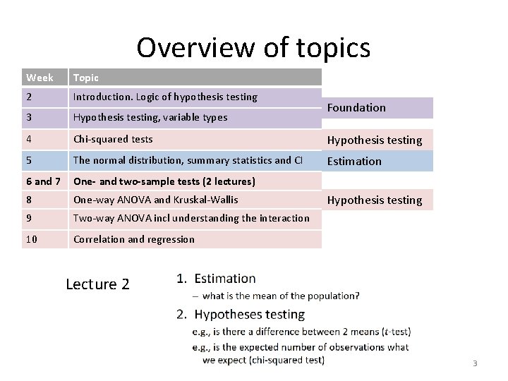
Overview of topics Week Topic 2 Introduction. Logic of hypothesis testing 3 Hypothesis testing, variable types 4 Chi-squared tests Hypothesis testing 5 The normal distribution, summary statistics and CI Estimation 6 and 7 One- and two-sample tests (2 lectures) 8 One-way ANOVA and Kruskal-Wallis 9 Two-way ANOVA incl understanding the interaction 10 Correlation and regression Foundation Hypothesis testing Lecture 2 3

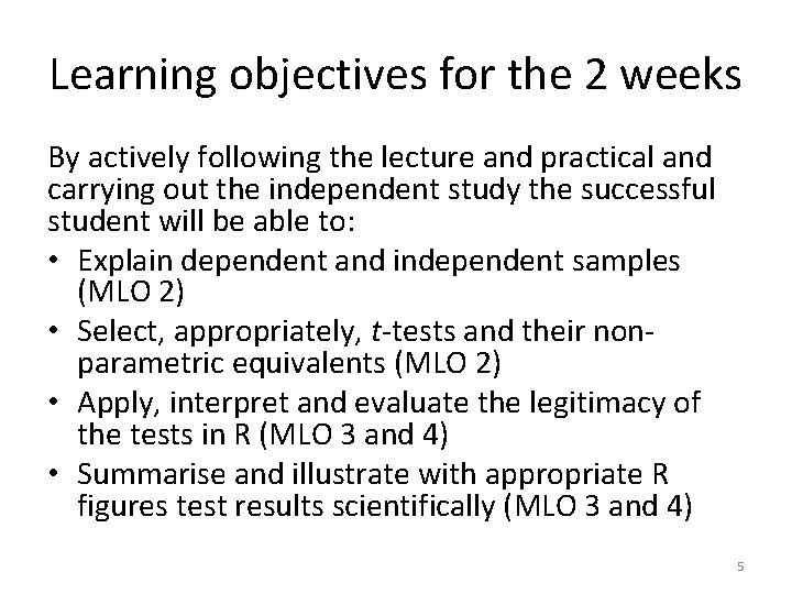
Learning objectives for the 2 weeks By actively following the lecture and practical and carrying out the independent study the successful student will be able to: • Explain dependent and independent samples (MLO 2) • Select, appropriately, t-tests and their nonparametric equivalents (MLO 2) • Apply, interpret and evaluate the legitimacy of the tests in R (MLO 3 and 4) • Summarise and illustrate with appropriate R figures test results scientifically (MLO 3 and 4) 5

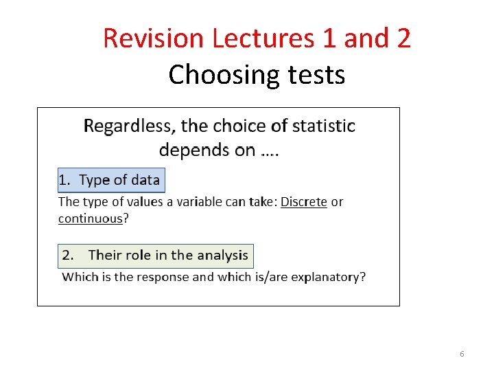
Revision Lectures 1 and 2 Choosing tests 6

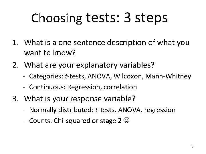
Choosing tests: 3 steps 1. What is a one sentence description of what you want to know? 2. What are your explanatory variables? - Categories: t-tests, ANOVA, Wilcoxon, Mann-Whitney - Continuous: Regression, correlation 3. What is your response variable? - Normally distributed: t-tests, ANOVA, regression - Counts: Chi-squared or stage 2 7

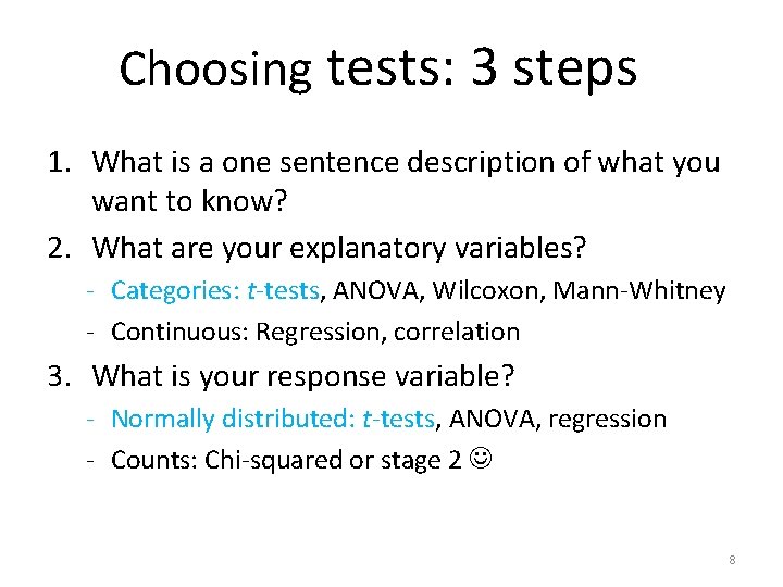
Choosing tests: 3 steps 1. What is a one sentence description of what you want to know? 2. What are your explanatory variables? - Categories: t-tests, ANOVA, Wilcoxon, Mann-Whitney - Continuous: Regression, correlation 3. What is your response variable? - Normally distributed: t-tests, ANOVA, regression - Counts: Chi-squared or stage 2 8

Types of t-test 1. One-sample § Compares the mean of sample to a particular value (compares the response to a reference) • Includes paired-sample test – compares the mean difference to zero (i. e. , compares dependent means) 2. Two-sample § Compares two (independent) means to each other 9

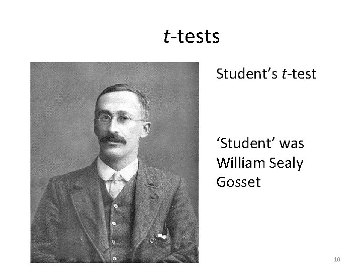
t-tests Student’s t-test ‘Student’ was William Sealy Gosset 10

t-tests in general Assumptions All t-tests assume the “residuals” are normally distributed and have homogeneity of variance A residual is the difference between the predicted and observed value Predicted value is the mean / group mean 11

t-tests in general: assumptions Checking Assumptions - Common sense – Data should be continuous – No/few repeats - Plot the residuals - Using a test in R 12

t-tests in general: assumptions When data are not normally distributed • Transform (not really covered) § E. g. Log to remove skew, arcsin squareroot on proportions • Use a non-parametric test (covered) § Fewer assumptions § Generally less powerful 13

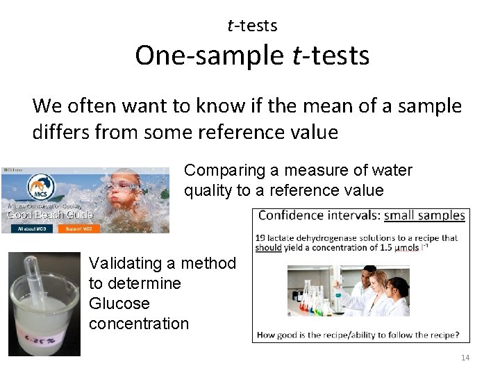
t-tests One-sample t-tests We often want to know if the mean of a sample differs from some reference value Comparing a measure of water quality to a reference value Validating a method to determine Glucose concentration 14

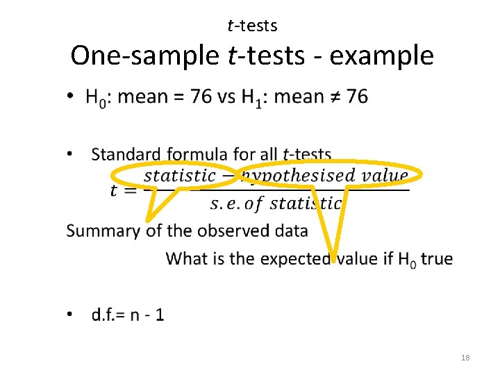
t-tests One-sample t-tests Tests whether the mean of a single sample differs from an expected value (i. e. , H 0) • Example: Fields are sprayed if crop plants have a disease score* of 76. • 20 plants in a field are measured • Is their mean significantly different from the reference of 76? *Arbitrary scale 15

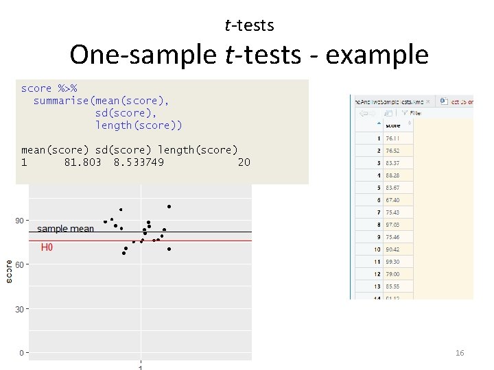
t-tests One-sample t-tests - example score %>% summarise(mean(score), sd(score), length(score)) mean(score) sd(score) length(score) 1 81. 803 8. 533749 20 16

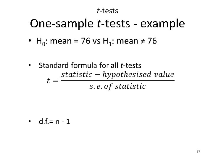
t-tests One-sample t-tests - example • 17

t-tests One-sample t-tests - example • 18

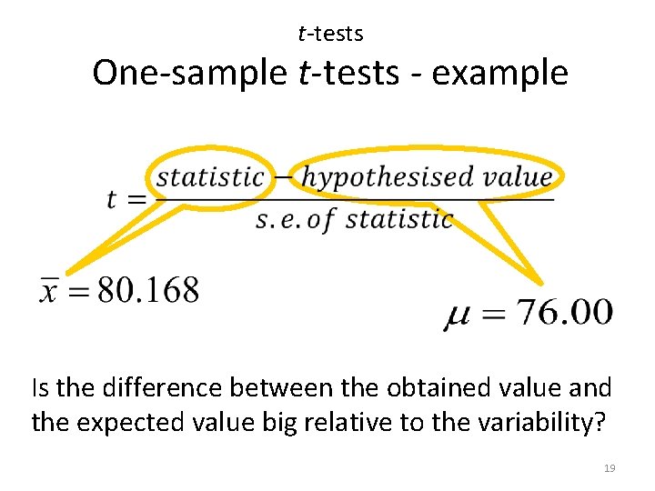
t-tests One-sample t-tests - example Is the difference between the obtained value and the expected value big relative to the variability? 19

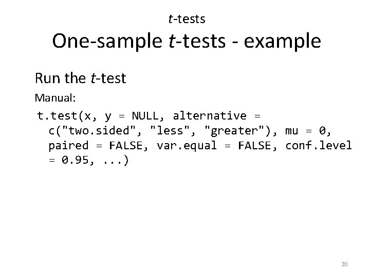
t-tests One-sample t-tests - example Run the t-test Manual: t. test(x, y = NULL, alternative = c("two. sided", "less", "greater"), mu = 0, paired = FALSE, var. equal = FALSE, conf. level = 0. 95, . . . ) 20

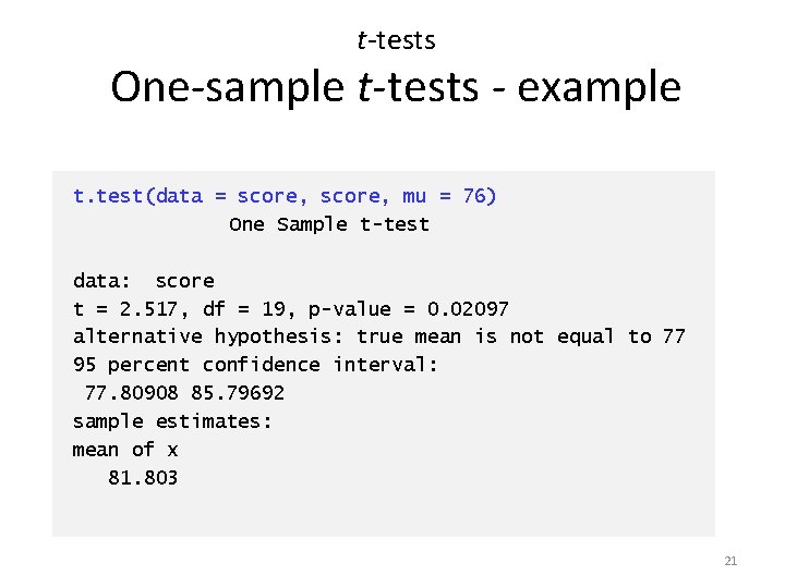
t-tests One-sample t-tests - example t. test(data = score, mu = 76) One Sample t-test data: score t = 2. 517, df = 19, p-value = 0. 02097 alternative hypothesis: true mean is not equal to 77 95 percent confidence interval: 77. 80908 85. 79692 sample estimates: mean of x 81. 803 21

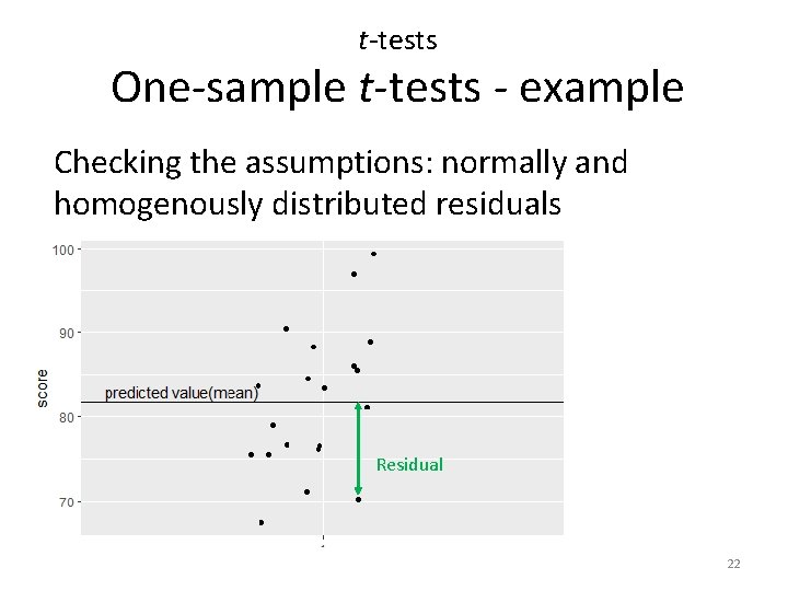
t-tests One-sample t-tests - example Checking the assumptions: normally and homogenously distributed residuals Residual 22

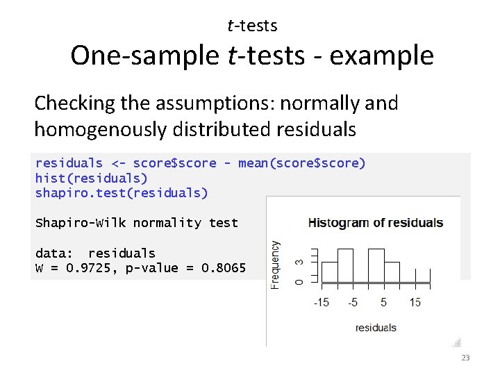
t-tests One-sample t-tests - example Checking the assumptions: normally and homogenously distributed residuals <- score$score - mean(score$score) hist(residuals) shapiro. test(residuals) Shapiro-Wilk normality test data: residuals W = 0. 9725, p-value = 0. 8065 23

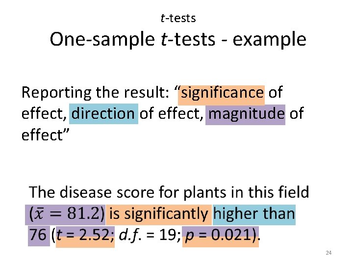
t-tests One-sample t-tests - example Reporting the result: “significance of effect, direction of effect, magnitude of effect” • 24

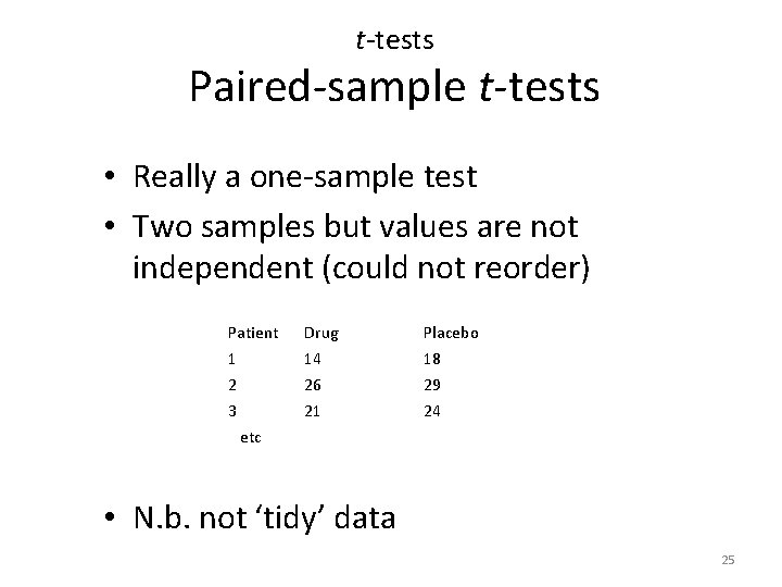
t-tests Paired-sample t-tests • Really a one-sample test • Two samples but values are not independent (could not reorder) Patient 1 2 3 etc Drug 14 26 21 Placebo 18 29 24 • N. b. not ‘tidy’ data 25

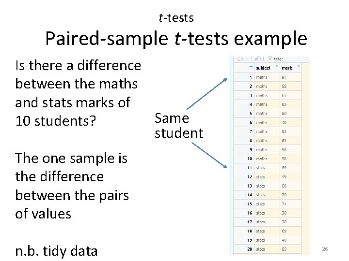
t-tests Paired-sample t-tests example Is there a difference between the maths and stats marks of Same 10 students? student The one sample is the difference between the pairs of values n. b. tidy data 26

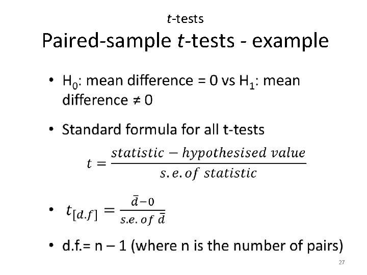
t-tests Paired-sample t-tests - example • 27

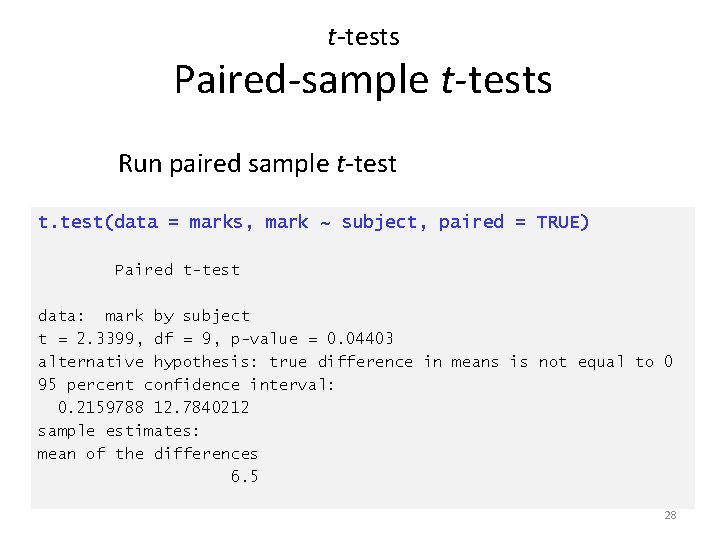
t-tests Paired-sample t-tests Run paired sample t-test t. test(data = marks, mark ~ subject, paired = TRUE) Paired t-test data: mark by subject t = 2. 3399, df = 9, p-value = 0. 04403 alternative hypothesis: true difference in means is not equal to 0 95 percent confidence interval: 0. 2159788 12. 7840212 sample estimates: mean of the differences 6. 5 28

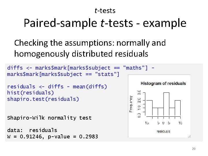
t-tests Paired-sample t-tests - example Checking the assumptions: normally and homogenously distributed residuals diffs <- marks$mark[marks$subject == "maths"] marks$mark[marks$subject == "stats"] residuals <- diffs - mean(diffs) hist(residuals) shapiro. test(residuals) Shapiro-Wilk normality test data: residuals W = 0. 91246, p-value = 0. 2983 29

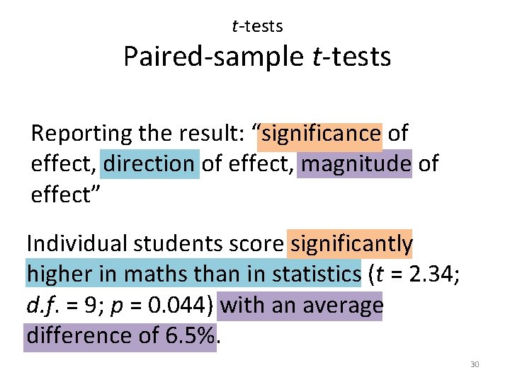
t-tests Paired-sample t-tests Reporting the result: “significance of effect, direction of effect, magnitude of effect” Individual students score significantly higher in maths than in statistics (t = 2. 34; d. f. = 9; p = 0. 044) with an average difference of 6. 5%. 30

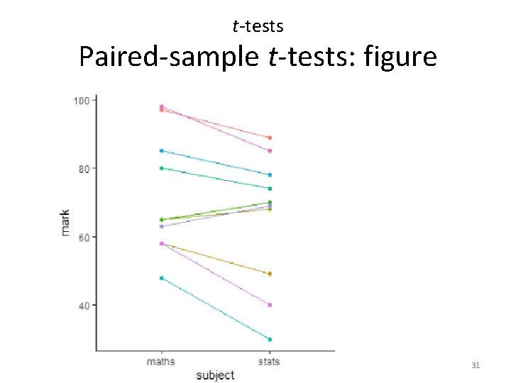
t-tests Paired-sample t-tests: figure 31

When the t-test assumptions are not met: non- parametric tests • Non-parametric tests make fewer assumptions • Based on the ranks rather than the actual data • Null hypotheses are about the mean rank (not the mean) 32

Non-parametric tests t-test equivalents i, . e. , the type of question is the same but the response variable is not normally distributed or it is impossible to tell (small samples) • one – sample t-test and paired-sample t-test: the one-sample Wilcoxon • Two-sample t-test (next lecture): two-sample Wilcoxon aka Mann-Whitney 33

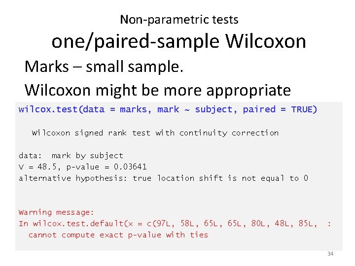
Non-parametric tests one/paired-sample Wilcoxon Marks – small sample. Wilcoxon might be more appropriate wilcox. test(data = marks, mark ~ subject, paired = TRUE) Wilcoxon signed rank test with continuity correction data: mark by subject V = 48. 5, p-value = 0. 03641 alternative hypothesis: true location shift is not equal to 0 Warning message: In wilcox. test. default(x = c(97 L, 58 L, 65 L, 80 L, 48 L, 85 L, cannot compute exact p-value with ties : 34

Non-parametric tests one/paired-sample Wilcoxon Reporting the result: “significance of effect, direction of effect, magnitude of effect” Individual students score significantly higher in maths than in statistics (Wilcoxon: V = 48. 5; n = 10; p = 0. 036) with a median difference of 7. 5%. 35

Learning objectives for the week By attending the lectures and practical the successful student will be able to • Explain dependent and independent samples (MLO 2) • Select, appropriately, t-tests and their nonparametric equivalents (MLO 2) • Apply, interpret and evaluate the legitimacy of the tests in R (MLO 3 and 4) • Summarise and illustrate with appropriate R figures test results scientifically (MLO 3 and 4) 36