Labor Economics Exercise session 1 Random data generation
Labor Economics Exercise session # 1 Random data generation Jan Matuska November, 2006
Overview: Graphing Generating random variables Generating random dummy variables from sample Drawing from multivariate distributions Throwing seeds Loops and distribution of estimated coefficients
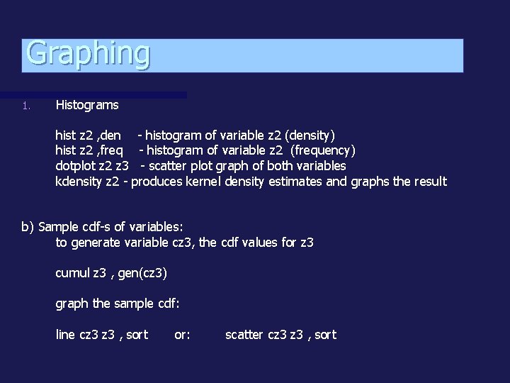
Graphing 1. Histograms hist z 2 , den - histogram of variable z 2 (density) hist z 2 , freq - histogram of variable z 2 (frequency) dotplot z 2 z 3 - scatter plot graph of both variables kdensity z 2 - produces kernel density estimates and graphs the result b) Sample cdf-s of variables: to generate variable cz 3, the cdf values for z 3 cumul z 3 , gen(cz 3) graph the sample cdf: line cz 3 , sort or: scatter cz 3 , sort
![Generating random variables 1 500 draws from the uniform distribution on [0, 1] set Generating random variables 1 500 draws from the uniform distribution on [0, 1] set](http://slidetodoc.com/presentation_image_h2/535b9a6e6fb955e55a46e751df268526/image-4.jpg)
Generating random variables 1 500 draws from the uniform distribution on [0, 1] set obs 500 gen x 1 = uniform() 500 draws from the standard normal distribution, mean 0, variance 1 gen x 2 = invnorm(uniform()) 500 draws from the distribution N(1, 2) gen x 3 = 1 + 4*invnorm(uniform())
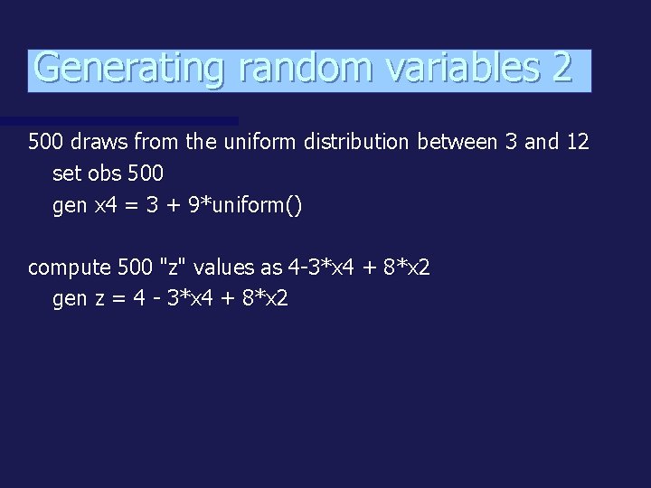
Generating random variables 2 500 draws from the uniform distribution between 3 and 12 set obs 500 gen x 4 = 3 + 9*uniform() compute 500 "z" values as 4 -3*x 4 + 8*x 2 gen z = 4 - 3*x 4 + 8*x 2
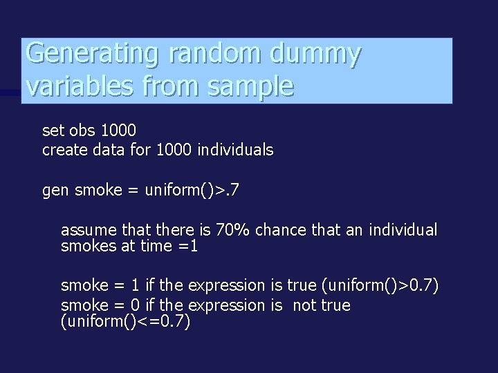
Generating random dummy variables from sample set obs 1000 create data for 1000 individuals gen smoke = uniform()>. 7 assume that there is 70% chance that an individual smokes at time =1 smoke = 1 if the expression is true (uniform()>0. 7) smoke = 0 if the expression is not true (uniform()<=0. 7)
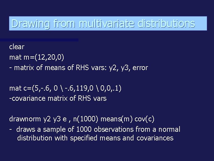
Drawing from multivariate distributions clear mat m=(12, 20, 0) - matrix of means of RHS vars: y 2, y 3, error mat c=(5, -. 6, 0 -. 6, 119, 0 0, 0, . 1) -covariance matrix of RHS vars drawnorm y 2 y 3 e , n(1000) means(m) cov(c) - draws a sample of 1000 observations from a normal distribution with specified means and covariances
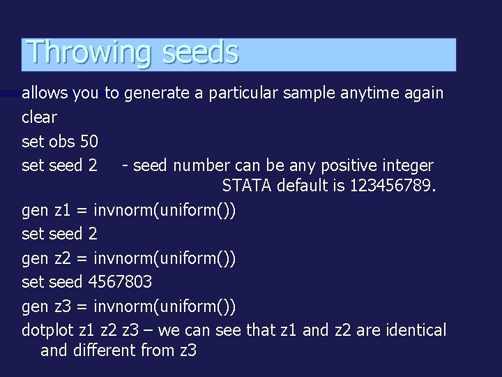
Throwing seeds allows you to generate a particular sample anytime again clear set obs 50 set seed 2 - seed number can be any positive integer STATA default is 123456789. gen z 1 = invnorm(uniform()) set seed 2 gen z 2 = invnorm(uniform()) set seed 4567803 gen z 3 = invnorm(uniform()) dotplot z 1 z 2 z 3 – we can see that z 1 and z 2 are identical and different from z 3
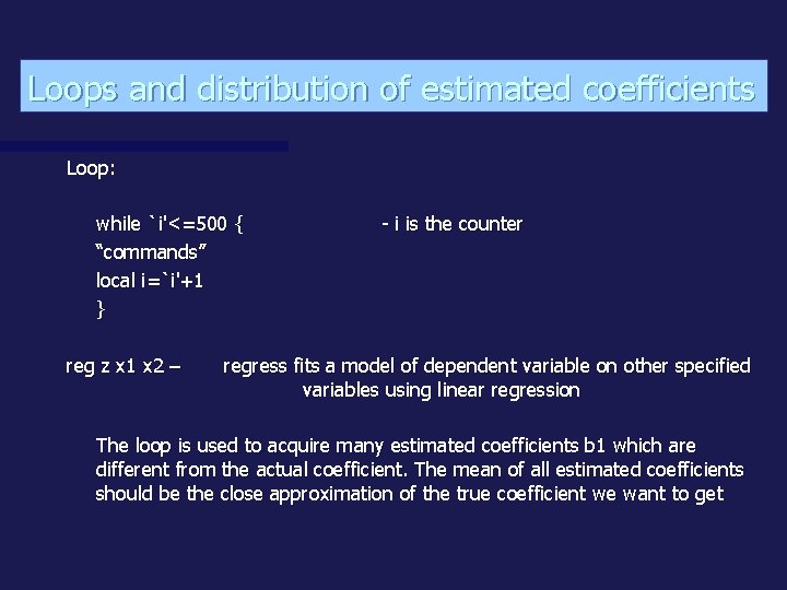
Loops and distribution of estimated coefficients Loop: while `i'<=500 { “commands” local i=`i'+1 } reg z x 1 x 2 – - i is the counter regress fits a model of dependent variable on other specified variables using linear regression The loop is used to acquire many estimated coefficients b 1 which are different from the actual coefficient. The mean of all estimated coefficients should be the close approximation of the true coefficient we want to get

Thank you for attention
- Slides: 10