Lab 6 The Fourier Transform How to transform

Lab 6: The Fourier Transform

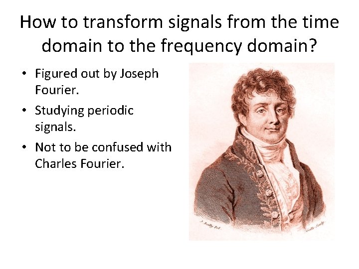
How to transform signals from the time domain to the frequency domain? • Figured out by Joseph Fourier. • Studying periodic signals. • Not to be confused with Charles Fourier.

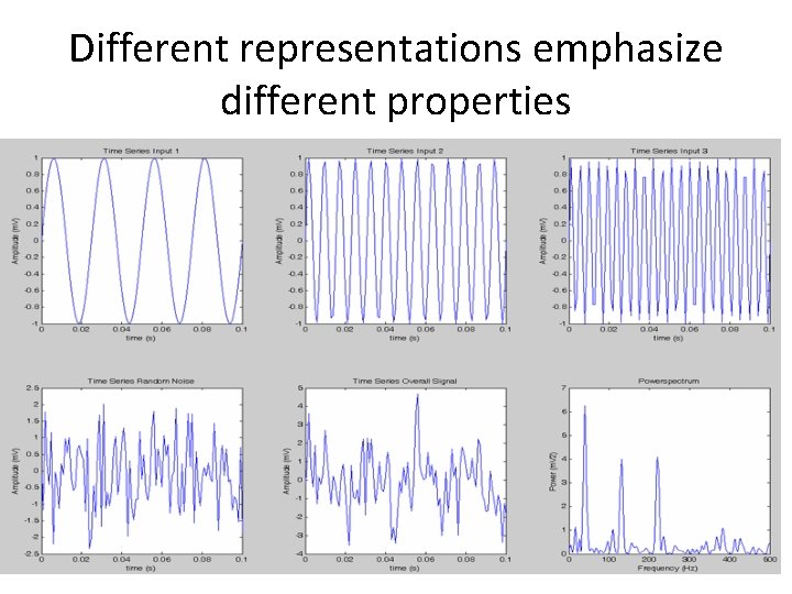
Different representations emphasize different properties

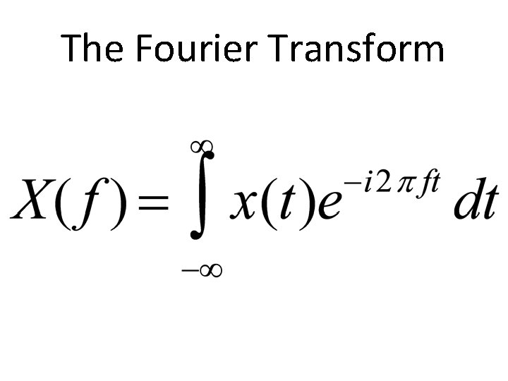
The Fourier Transform

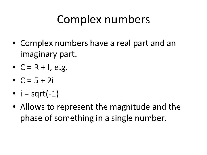
Complex numbers • Complex numbers have a real part and an imaginary part. • C = R + I, e. g. • C = 5 + 2 i • i = sqrt(-1) • Allows to represent the magnitude and the phase of something in a single number.

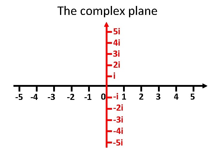
The complex plane 5 i 4 i 3 i 2 i i -5 -4 -3 -2 -1 0 -i 1 -2 i -3 i -4 i -5 i 2 3 4 5

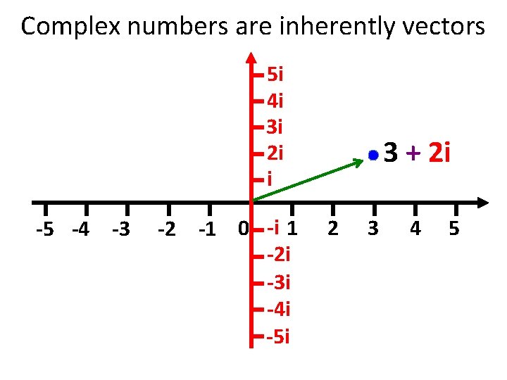
Complex numbers are inherently vectors 5 i 4 i 3 i 2 i i -5 -4 -3 -2 -1 0 -i 1 -2 i -3 i -4 i -5 i 3 + 2 i 2 3 4 5

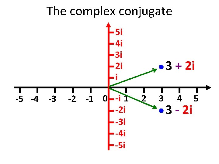
The complex conjugate 5 i 4 i 3 i 2 i i -5 -4 -3 -2 -1 0 -i 1 -2 i -3 i -4 i -5 i 3 + 2 i 2 3 4 3 - 2 i 5

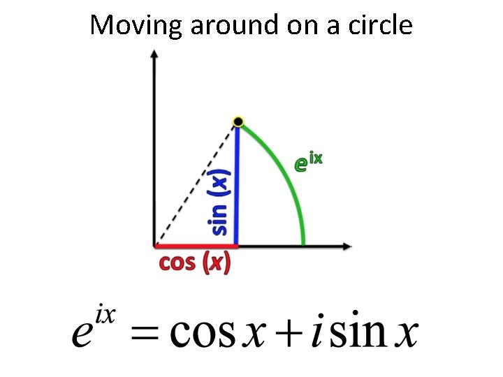
Moving around on a circle

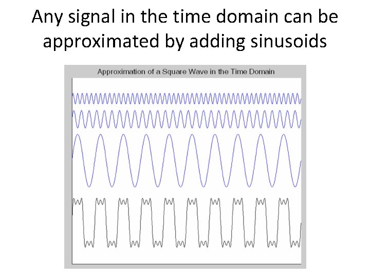
Any signal in the time domain can be approximated by adding sinusoids

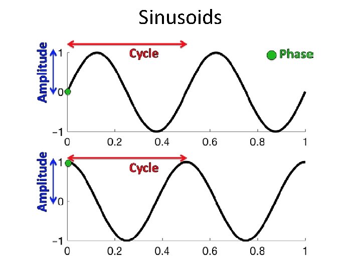
Sinusoids

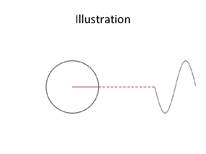
Illustration

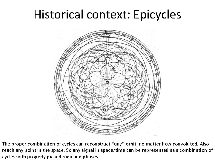
Historical context: Epicycles The proper combination of cycles can reconstruct *any* orbit, no matter how convoluted. Also reach any point in the space. So any signal in space/time can be represented as a combination of cycles with properly picked radii and phases.

Game changers: 1 - FFT • Original Fourier Transform has been known since early 19 th century. • “Fast Fourier Transform” does a discrete Fourier Transform. • It is fast. • Given modern computers, it is even faster. • Fourier Transform becomes useful

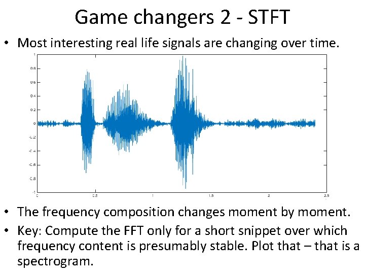
Game changers 2 - STFT • Most interesting real life signals are changing over time. • The frequency composition changes moment by moment. • Key: Compute the FFT only for a short snippet over which frequency content is presumably stable. Plot that – that is a spectrogram.

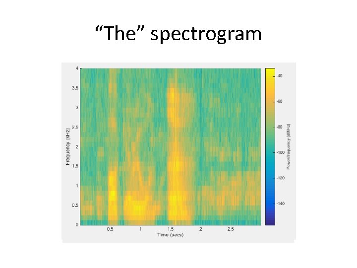
“The” spectrogram

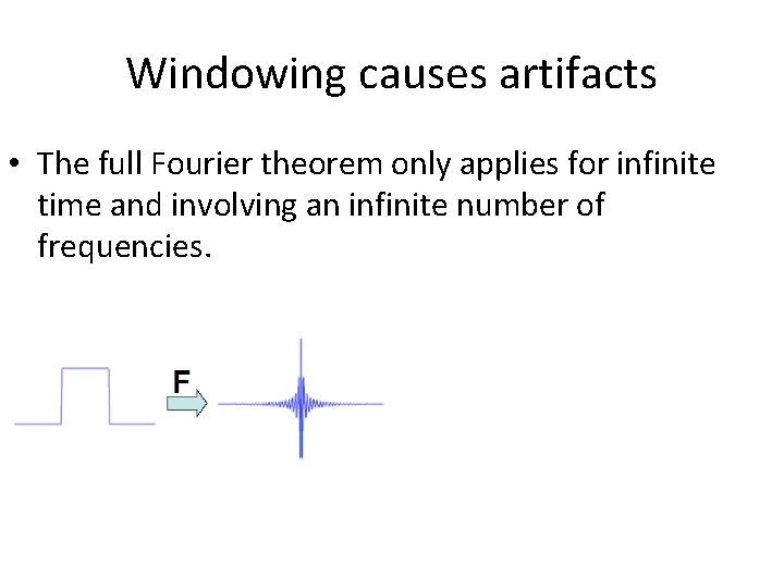
Windowing causes artifacts • The full Fourier theorem only applies for infinite time and involving an infinite number of frequencies.

Aliasing: The Nyquist frequency • The maximal frequency that one can represent without aliasing the signal is the “Nyquist frequency”. • It corresponds to half the sampling rate. • We’ll do stuff in Matlab to understand this. • First: The GUI