Lab 6 Last lab Basin Hopping General goal
: Basin Hopping")
Lab 6 (Last lab!): Basin Hopping

General goal of global optimization • Find the global optimization faster. • What is the limitation of MD for global optimization?

Molecular Dynamics • Molecular Dynamics numerical integrates Newton’s Equations of motion, – F=ma – v=dr/dt – etc. • To simulate movement of atoms over time • We also introduced ensembles where we fix thermodynamic variables – Canonical Ensemble (NVT) – Microcanonical Ensemble (NVE)
 Starting Point r 1) Start at high temperature to allow sampling")
Simulated Annealing V(r) Starting Point r 1) Start at high temperature to allow sampling of full PES
 Starting Point r 1) Start at high temperature to allow sampling")
Simulated Annealing V(r) Starting Point r 1) Start at high temperature to allow sampling of full PES 2) Then, lower the temperature according to a cooling schedule
 V(r) Starting Point Ending Point r 1) Start at high temperature")
Simulated Annealing (SA) V(r) Starting Point Ending Point r 1) Start at high temperature to allow sampling of full PES 2) Then, lower the temperature according to a cooling schedule 3) End at hopefully lower energy than where you started; SA doesn’t guarantee hitting the global minimum

Simulated Annealing • Lab 5 -Part 2 you will select your own cooling schedule.

Problems with simulated annealing • With a canonical ensemble: what would happen if the temperature is too low or too high? V(r) Starting Point r

Problems with simulated annealing • If temperature is too low, the structures that you can discovered is limited as there will be barriers that you can’t overcome. V(r) If your KE (temperature) is not higher than this Then you cannot pass this barrier. Why? Starting Point r

Problems with simulated annealing • If temperature is too high, the number of structures that you can possibly find is too Then you could end For global large. up somewhere to optimization, is V(r) If your KE (temperature) is not higher than this Starting Point the left of this barrier. microcanonical ensemble even useful? How could thermostat settings, such as collision chance, impact the simulation? r How could total simulation time impact our chance of finding the global minimum?

Problems with simulated annealing • Imagine how many force calls is needed till we arrive at the global minimum. • Imagine how many of the force calls are repetitive. V(r) Starting Point r

Global Optimization Potential Energy • Wouldn't it be ideal if we don’t have to spend as much time climbing each the barriers? Local Minimum hop Global Minimum Molecular Coordinates

Basin Hopping • 1. Start with an initial structure R. Optimize this structure to get Ropt with P(Ropt)=e-V(Ropt)/k. T and potential energy V(Ropt) R Ropt

Basin Hopping • 2. Generate a new structure R’. Optimize this structure to get Ropt’ with P(Ropt’)=e-V(Ropt’)/k. T and potential energy V(Ropt’) R R’ Ropt R’opt
 >= P(Ropt): • Accept this configuration R =R’ Ropt")
Basin Hopping • If P(Ropt’) >= P(Ropt): • Accept this configuration R =R’ Ropt R’opt

Basin Hopping • 1. Start with an initial structure R. Optimize this structure to get Ropt with P(Ropt)=e-V(Ropt)/k. T and potential energy V(Ropt) R Ropt

Basin Hopping • 2. Generate a new structure R’. Optimize this structure to get Ropt’ with P(Ropt’)=e-V(Ropt’)/k. T and potential energy V(Ropt’) R’ R R’opt Ropt
 >= P(R): Accept this configuration Else: R’ R R’opt Ropt")
Basin Hopping If P(R’) >= P(R): Accept this configuration Else: R’ R R’opt Ropt

Basin Hopping Generate a random number between 0 and 1 called RAND • if e-(V(Ropt’)-V(Ropt))/k. T > RAND: Accept this configuration • Else: reject R’ R R’opt Ropt

Metropolis Monte Carlo for Basin Hopping 1. Start with an initial structure R. Optimize this structure to get R opt with P(Ropt)=e-V(Ropt)/k. T and potential energy V(Ropt) 2. Generate a new structure R’. Optimize this structure to get R opt’ with P(Ropt’)=e-V(Ropt’)/k. T and potential energy V(Ropt’) If P(Ropt’) >= P(Ropt): Accept this configuration i. e. R = R’ If P(Ropt’) < P(Ropt): Generate a random number between 0 and 1 called RAND if e-(V(Ropt’)-V(Ropt))/k. T > RAND: Accept this configuration i. e. R = R’ REPEAT THIS PROCEDURE MANY TIMES TO GET A SERIES OF POINTS FROM A PROBABILITY DISTRUBTION

Random Moves • How to create new configurations? – R R’ • This can be from any distribution you choose! • You will get the opportunity to select a distribution of you choice in the next lab

This is the information required for your next lab… Questions?
 the canonical ensemble (NVT)")
Boltzmann Distribution Probability of finding a molecular configuration in V(r) the canonical ensemble (NVT) P(r) r
 the canonical ensemble (NVT)")
Boltzmann Distribution Probability of finding a molecular configuration in V(r) the canonical ensemble (NVT) P(r) If you run a NVT trajectory you will sample the Boltzmann Distribution r

Monte Carlo Methods • In this course we have talked about some numerical methods: – Methods for local optimization • Gradient Descent and Newton’s Method – Euler’s method used in molecular dynamics simulations – Reimann Sum

Monte Carlo Methods • In this course we have talked about some numerical methods: – Methods for local optimization • Gradient Descent and Newton’s Method – Euler’s method used in molecular dynamics simulations – Reimann Sum • Today we will add to that tool kit by talk about how we can also use random numbers to solve quantitative problems – Methods for which utilize random numbers are known as Monte Carlo methods

How can we use random numbers to solve quantitative problems? 2 • Procedure for calculating π: 2
")
How can we use random numbers to solve quantitative problems? (0. 46, 1. 16) • Procedure for calculating π: • Select two uniform random numbers between 0 and 2 for x and y coordinates • Label the point as in (red) or out (black) of the circle

How can we use random numbers to solve quantitative problems? • Procedure for calculating π: • Select two uniform random numbers between 0 and 2 for x and y coordinates • Label the point as in (red) or out (black) of the circle • Repeat many times

How can we use random numbers to solve quantitative problems?

How can we use random numbers to solve quantitative problems?

How can we use random numbers to solve quantitative problems?

How can we use random numbers to solve quantitative problems? • This is a away of approximately finding area or doing numerical integration. • Accuracy of the value of Pi depends on the number of random points used • This is not more efficient for calculating Pi than other numerical methods such as a Reimann Sum

Dimensionality • What would happened to the expense of using a Reimann Sum to find the area of a sphere? – Number of samples require scales exponentially with dimension N samples required N N 2 samples required

Dimensionality • What would happened to the expense of using a Monte Carlo method like the previous example to find the area of a sphere? – Same as a Reimann Sum! Exponential scaling with dimension! N 2 samples required N 3 samples required

Metropolis Monte Carlo • A method for obtaining a random sequence of configurations from a probability distribution when sampling is difficult (high dimensional systems)

Metropolis Monte Carlo • A method for obtaining a random sequence of configurations from a probability distribution when sampling is difficult (high dimensional systems) • First I will give an example of how this can be useful • Then, I will first introduce the procedure of the algorithm • I have left out the derivation of this method

Metropolis Monte Carlo • A method for obtaining a random sequence of configurations from a probability distribution when sampling is difficult (high dimensional systems) • How could we use this?

Metropolis Monte Carlo • A method for obtaining a random sequence of configurations from a probability distribution when sampling is difficult (high dimensional systems) • How could we use this? • There are many applications but one example could be the average potential energy of a system • Here is one way of calculating the average potential energy V(r) r

Metropolis Monte Carlo • A method for obtaining a random sequence of configurations from a probability distribution when sampling is difficult (high dimensional systems) • How could we use this? • There are many applications but one example could be the average potential energy of a system • We could also use MC V(r) P(r) Where V(r) is selected from the Probability distribution P(r) r

Metropolis Monte Carlo • A method for obtaining a random sequence of configurations from a probability distribution when sampling is difficult (high dimensional systems) • How could we use this? • There are many applications but one example could be the average potential energy of a system • We could also use MC Metropolis Monte Carlo is superior for High Dimensional Systems!
=e-V(R)/k. T and")
Metropolis Monte Carlo 1. Start with an initial structure R with P(R)=e-V(R)/k. T and potential energy V(R) Boltzmann Distribution R
 and")
Metropolis Monte Carlo 1. Start with an initial structure R with energy V(R) and probabilty P(R) 2. Generate a new structure R’ with energy V(R’) and probability P(R)=e-V(R’)/k. T R, P(R) R’, P(R’)
=e-V(R)/k. T and")
Metropolis Monte Carlo 1. Start with an initial structure R with P(R)=e-V(R)/k. T and potential energy V(R) 2. Generate a new structure R’ with energy V(R’) and probability P(R)=e-V(R’)/k. T If P(R’) >= P(R): Accept this configuration i. e. R = R’ V(R’) < V(R) so accept this position! R, P(R) R’, P(R’)
=e-V(R)/k. T and")
Metropolis Monte Carlo 1. Start with an initial structure R with P(R)=e-V(R)/k. T and potential energy V(R) 2. Generate a new structure R’ with energy V(R’) and probability P(R)=e-V(R’)/k. T If P(R’) >= P(R): Accept this configuration i. e. R = R’ R’, P(R’) V(R’) > V(R) so need to move on… R, P(R)
=e-V(R)/k. T and")
Metropolis Monte Carlo 1. Start with an initial structure R with P(R)=e-V(R)/k. T and potential energy V(R) 2. Generate a new structure R’ with energy V(R’) and probability P(R)=e-V(R’)/k. T Else: Generate a random number between 0 and 1 called RAND if e-(V(R’)-V(R))/k. T > RAND: Accept this configuration i. e. R = R’ R’, P(R’) R, P(R)
=e-V(R)/k. T and")
Metropolis Monte Carlo 1. Start with an initial structure R with P(R)=e-V(R)/k. T and potential energy V(R) 2. Generate a new structure R’ with energy V(R’) and probability P(R)=e-V(R’)/k. T RAND=0. 23 If P(R’) < P(R) or V(R’) > V(R): Generate a random number between 0 and 1 called RAND if e-(V(R’)-V(R))/k. T > RAND: Accept this configuration i. e. R = R’ e-(V(R’)-V(R))/k. T =P(R’)/P(R)=0. 07 R’, P(R’) R, P(R)
=e-V(R)/k. T and")
Metropolis Monte Carlo 1. Start with an initial structure R with P(R)=e-V(R)/k. T and potential energy V(R) 2. Generate a new structure R’ with energy V(R’) and probability P(R)=e-V(R’)/k. T RAND=0. 23 If P(R’) < P(R) or V(R’) > V(R): Generate a random number between 0 and 1 called RAND if e-(V(R’)-V(R))/k. T > RAND: Accept this configuration i. e. R = R’ e-(V(R’)-V(R))/k. T =P(R’)/P(R)=0. 07 So, Reject this configuration! R’, P(R’) R, P(R)

Metropolis Monte Carlo for the Boltzmann Distribution 1. Start with an initial structure R with P(R)=e-V(R)/k. T and potential energy V(R) 2. Generate a new structure R’ with energy V(R’) and probability P(R)=e-V(R’)/k. T If PV(R’) <= V(R): Accept this configuration i. e. R = R’ El. If V(R’) > V(R): Generate a random number between 0 and 1 called RAND if e-(V(R’)-V(R))/k. T > RAND: Accept this configuration i. e. R = R’ REPEAT THIS PROCEDURE MANY TIMES TO GET A SERIES OF POINTS FROM A PROBABILITY DISTRUBTION

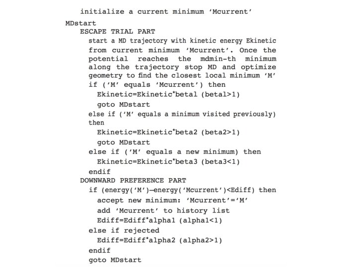
Fixed Parameters: Beta 1 Beta 2 Beta 3 Alpha 1 Alpha 2 Dynamic Parameters: Ediff Ekinetic Minima Hopping Mcurrent To start the Minima Hopping algorithm, pick the following initial conditions: • Mcurrent • Kinetic energy (Ekinetic)

Fixed Parameters: Beta 1 Beta 2 Beta 3 Alpha 1 Alpha 2 Dynamic Parameters: Ediff Ekinetic Minima Hopping Mcurrent • Start a NVE MD trajectory with kinetic energy Ekinetic • Once you pass a minimum mdmin = 2 stop the trajectory and optimize your structure to obtain a Mnew

Fixed Parameters: Beta 1 Beta 2 Beta 3 Alpha 1 Alpha 2 Dynamic Parameters: Ediff Ekinetic Minima Hopping Mcurrent=Mnew If Mnew= Mcurrent: Increase Ekinetic=Ekinetic *beta 1 where beta 1 > 0

Fixed Parameters: Beta 1 Beta 2 Beta 3 Alpha 1 Alpha 2 Dynamic Parameters: Ediff Ekinetic Minima Hopping Mcurrent • Start a NVE MD trajectory with kinetic energy Ekinetic • Once you pass a minimum mdmin = 2 stop the trajectory and optimize your structure to obtain a Mnew

Fixed Parameters: Beta 1 Beta 2 Beta 3 Alpha 1 Alpha 2 Dynamic Parameters: Ediff Ekinetic Minima Hopping Mcurrent Mnew If Mnew= Mcurrent: Increase Ekinetic=Ekinetic *beta 1 where beta 1 > 0 Else: Decrease Ekinetic=Ekinetic *beta 3 where beta 3 < 0

Fixed Parameters: Beta 1 Beta 2 Beta 3 Alpha 1 Alpha 2 Dynamic Parameters: Ediff Ekinetic E Minima Hopping diff Mcurrent Mnew If (V(Mnew) – V(Mcurrent)) < Ediff: Accept new minimum; Mcurrent=Mnew Add Mcurrent to history Ediff = Ediff*alpha 1 where alpha 1 < 0

Fixed Parameters: Beta 1 Beta 2 Beta 3 Alpha 1 Alpha 2 Dynamic Parameters: Ediff Ekinetic Minima Hopping Mcurrent If Mnew= Mcurrent: Increase Ekinetic=Ekinetic *beta 1 where beta 1 > 0

Fixed Parameters: Beta 1 Beta 2 Beta 3 Alpha 1 Alpha 2 Dynamic Parameters: Ediff Ekinetic Minima Hopping Mnew Mcurrent If Mnew= Mcurrent: Increase Ekinetic=Ekinetic *beta 1 where beta 1 > 0 Elif Mnew is a previously visited minimum: Increase Ekinetic=Ekinetic *beta 2 where beta 2 > 0 Else: Decrease Ekinetic=Ekinetic *beta 3 where beta 3 < 0

Fixed Parameters: Beta 1 Beta 2 Beta 3 Alpha 1 Alpha 2 Dynamic Parameters: Ediff Ekinetic Minima Hopping Mcurrent If Mnew= Mcurrent: Increase Ekinetic=Ekinetic *beta 1 where beta 1 > 0 Elif Mnew is a previously visited minimum: Increase Ekinetic=Ekinetic *beta 2 where beta 2 > 0 Else: Decrease Ekinetic=Ekinetic *beta 3 where beta 3 < 0

Fixed Parameters: Beta 1 Beta 2 Beta 3 Alpha 1 Alpha 2 Dynamic Parameters: Ediff Ekinetic Minima Hopping Mnew Ediff Mcurrent If (V(Mnew) – V(Mcurrent)) < Ediff: Accept new minimum; Mcurrent=Mnew Else: Reject this minimum and increase Ediff = Ediff*alpha 2

Comparison of Minima and Basin Hopping Method Basin Hopping Minima Hopping Trial Move Acceptance Critieria History Random Metropolis Monte displacement Carlo Molecular Dynamics (V(Mnew) – V(Mcurrent)) < Ediff Reject a state and increase kinetic energy if

Benefits of Minima Hopping • Molecular dynamics tends to go to low energy local minima close by while random displacements do not necessarily find low energy minima

Benefits of Minima Hopping • Molecular dynamics tends to go to low energy local minima close by while random displacements do not necessarily find low energy minima • Changes the acceptance criteria and kinetic energy to dynamically change to escape out of funnels

That’s it!

Lab 1 Feedback

Lab 1 Feedback • Difference between Newton Method’s wiki page and Newton Methods • Newton’s Method wiki – Method used for finding roots of functions – Perfect for linear functions g(x) x 0 x 1 x

Lab 1 Feedback • Newton’s Method in Optimization – Newton’s Method used for finding roots of functions – In optimization we want to find the root of the derivative – So, perfect for harmonic functions V(x) x 1 x 0 x V’(x) x 1 x 0 x

Review: Methods for Local Optimization and Generating PES Class of Optimization Methods First Order Methods When to use this method? ASE/TSASE/PY THON VASP Far from minimum; Bad initial guess Gradient Descent IBRION=3 POTIM=0. 01 (similar to alpha) FIRE IBRION=2 SDLBFGS IBRION=1 Improved First Between the Order two extremes Second Order Close to minimum in quadratic region

Convergence Criteria 1 2 3 Convergence Criteria can be magnitude of entire force vector Or maximum force on all atoms But not, force from one atom

Extra Slides

Metropolis Monte Carlo • Where does this method come from? – Markov Chains: a random process that is memoryless – So you can make a prediction about the future based solely on where you currently are located from statistics – The criteria of a Markov Chain is
 R’, P(R’)")
Metropolis Monte Carlo R, P(R) R’, P(R’)
- Slides: 72