Lab 5 6 FollowUp More Python Images Images

Lab #5 -6 Follow-Up: More Python; Images
 is")
Images ● ● ● A signal (e. g. sound, temperature infrared sensor reading) is a single (onedimensional) quantity that varies over time. An image (picture) can be thought of as a two-dimensional quantity that varies over space. Otherwise, the computations for sounds and images are about the same!

Black-and-White Images
 whose")
● ● Eventually we get down to a single point (pixel, “picture element”) whose color we need to represent. For black-and-white images, two basic options – Halftone: Black (0) or white (1); having lots of points makes a region look gray – Grayscale: Some set of values (2 N, N typically = 8) representing shades of gray.

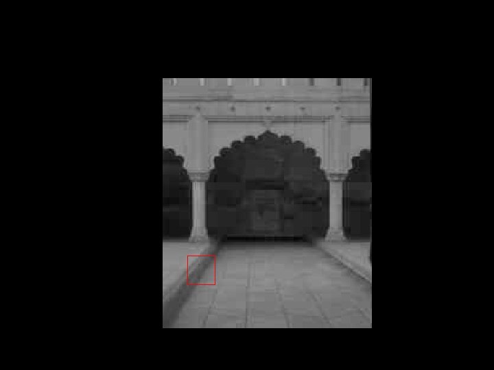
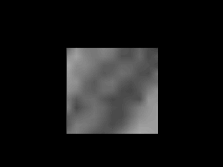
● To turn a b/w image into a grid of pixels, imagine running a stylus horizontally along the image:

● This gives us a one-dimensional function showing gray level at each point along the horizontal axis:

● Doing this repeatedly with lots of evenly-spaced scan lines gives us a grayscale map of the image: ● Height = grayscale value ● Spacing between lines = spacing within line
:")
Color ● Light comes in difference wavelengths (frequencies):
 can")
Like a sound, energy from a given light source (e. g. , star) can be described by its wavelength (frequency) spectrum : the amount of each wavelength present in the source. Intensity Energy (d. B) ● Frequency (Hz) Spectrum of vowel “ee” Wavelength (nm) Spectrum of star ICR 3287

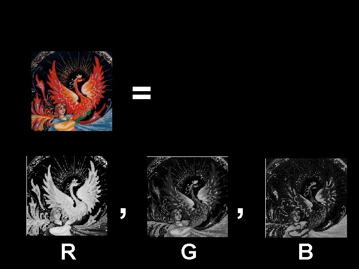
● ● Light striking our eyes is focused by a lens and projected onto the retina. The retina contains photoreceptors (sensors) called cones that respond to different wavelengths of light: red, green, and blue. So retina can be thought of as a transducer that inputs light and outputs a threedimensional value for each point in the image: [R, G, B], where R, G, and B each fall in the interval (0, 1). So we can represent any color image as three “grayscale” images:

Digital Sampling of Images ● ● ● Same questions arise for sampling images as for sound: – Sampling Frequency (how often to sample) – Quantization (# of bits per sample) With images, “how often” means “how many times per linear unit (inch, cm) – a. k. a. resolution (dpi) Focus on quantization – Each sample is either an RGB triple or an index into a color map – With too few bits, we lose gradual shading

Color Maps ● ● With 8 bits per color, 3 colors per pixel, we get 24 bits per pixel: 224 ≈ 17 million distinct colors We can actually get away with far fewer, using color maps Each pixel has a value that tells us what row in the color map to use Color map rows are R, G, B values:
 >> colormap ans = 0 0. . . 0. 4375")
Color Maps (in Matlab) >> colormap ans = 0 0. . . 0. 4375 0. 5000. . . 0. 5625 0. 5000 0 0 >> size(colormap) ans = 64 3 0 0 0. 5625 0. 6250 1. 0000 0. 5625 0. 5000 0 0

Quantization Problems With too few bits, we lose gradual shading: 1 bit 5 bits 2 bits 6 bits 3 bits 7 bits 4 bits 8 bits

Sampling and Storing Images in Files • Cameras / scanners usually output images in one of several formats – JP(E)G (Joint Photographic Experts Group) – GIF (Graphics Interchange Format) – PNG (Portable Network Graphics) – TI(F)F (Tagged Image File Format) • As with sound formats, main issues in image formats are compression scheme (how images are stored and transmitted to save space/time) and copyright

JPEG Compression • Images contain lots of redundant information

• Images contain lots of redundant information 530 x 279 x 3 = 443610 bytes (assuming 3 bytes per pixel)

MOSTLY BLUE MOSTLY WHITE MOSTLY GREEN MOSTLY BROWN

Homebrew Compression

Homebrew Compression 530, 84, 151, 129, 235 530, 72, 255, 255 530, 66, 0, 128, 64 530, 60, 128, 64, 0

Homebrew Compression • Assuming two bytes per number 4*5*2 = 40 bytes • 443610 / 40 = factor of 11000! 530, 84, 151, 129, 235 530, 72, 255, 255 530, 66, 0, 128, 64 530, 60, 128, 64, 0

Lossy Compression • This sort of compression is lossy: reduces size but loses resolution • JPEG offers a better lossy compromise – typically, around factor 10 without noticeable loss in quality

The JPEG Algorithm 1. Convert each RGB pixel into a form in which brightness (“Luminance”) has its own value, and use just two values (“Chrominance”, red or blue) for color. http: //en. wikipedia. org/wiki/YCb. Cr

The JPEG Algorithm 2. Quantize the chroma data by a factor of two, because the eye is more sensitive to brightness than to color. E. g. : 83 98 123 200 44 01010011 01100010 01111011 11001000 00101100 01010000 01100000 0111000000 00100000 80 96 112 192 32

The JPEG Algorithm 3. Break the transformed image down into blocks of 8 x 8 pixels. We can represent each block as the weighted sum of various patterns, or frequency components, which will differ from block to block. The set of 64 weights becomes the new representation of the block. http: //en. wikipedia. org/wiki/JPEG#Discrete_cosine_transform
 to the")
The JPEG Algorithm 4. Quantize the frequency weights, giving more precision (bits) to the low-frequency components: again, because the eye is more sensitive to low-frequency variations (big, slowly changing patterns). JPEG Quality refers to how much we allow the high-frequency components to persist.

JPEG Quality Re-compressed with Quality = 0:

The JPEG Algorithm 5. Compress the quantized block weights using a lossless algorithm like Huffman Coding

Huffman Coding • The basic idea: Values that occur more often should be given shorter codes. • In the previous sentence:
: Values that occur … 11110001000010010011101 …")
So maybe use this code (ignoring space): Values that occur … 11110001000010010011101 …

Huffman Code • Uses a tree structure to determine when we’re at the end of a code item: http: //www. personal. kent. edu/~rmuhamma/Algorithms/My. Algorithms/Greedy/huffman. htm

Images: Summary • All digital data (MS Word files, JPEG images, MP 3 songs, MP 4 videos) is just a sequence of numbers • How we interpret those numbers depends on the program we’re using to look at the data • Compressions schemes (JPEG, MP 3) rely on ignoring the numbers that don’t make as much of a difference in our perception of the image, song, etc. • JPEG is not a single algorithm; it’s a grab-bag of techniques that yield good results in combination
- Slides: 35