Lab 08 CREATING VISUAL NARRATIVE Lecy Urban Policy

Lab 08 CREATING VISUAL NARRATIVE Lecy ∙ Urban Policy

COLOR FUNCTIONS

http: //colorbrewer 2. org/ color. vals <- c("#a 6611 a", "#dfc 27 d", "#f 5 f 5 f 5", "#80 cdc 1", "#018571" ) plot( 1: 5, c(5, 5, 5), col=color. vals, pch=19, cex=10, xlim=c(0, 6) )
 display. brewer. pal( 7, \"Br. BG\" ) display. brewer. pal(")
library( RColor. Brewer ) display. brewer. pal( 7, "Br. BG" ) display. brewer. pal( 5, "Br. BG" ) display. brewer. pal( 7, "Bu. Gn" ) brewer. pal( 5, "Br. BG" ) # identical to previous slide color. vals <- brewer. pal( 5, "Br. BG" )
 )")
color. function <- color. Ramp. Palette( c("firebrick 4", "light gray", "steel blue" ) ) color. function(5) # number of classes you desire col. vals <- color. function(7) plot( 1: 7, c(3, 3, 3, 3), pch=19, cex=10, col=col. vals, xlim=c(0, 8) )
 + 10 # Five groups, 20% of the data in")
norm. vec <- rnorm(10000) + 10 # Five groups, 20% of the data in each quantile( norm. vec, probs=c(0, 0. 20, 0. 40, 0. 60, 0. 80, 1 ), na. rm=T # Seven groups quantile( norm. vec, probs=seq( from=0, to=1, by=1/7 ), na. rm=T ) )

GRAPHICAL HIERARCHY
 to")
GROUND AND FIGURE • • Assign bright colors (red, orange, yellow, green, blue) to important graphic elements Features are known as figure, or the subject of the map. Assign drab colors to the graphic elements that provide orientation or context, especially shades of gray Features known as ground, or the context for the subject.

GOOD BAD

YOUR DATA TELLS A STORY

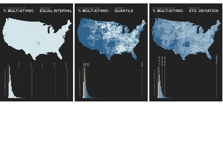
WHAT PATTERN DO YOU SEE?

WHAT PATTERN DO YOU SEE NOW? Equal Intervals Quantiles These maps are all made with the same data using different intervals for the break points. Geometric

BREAK POINTS FOR NORMAL DISTRIBUTIONS http: //uxblog. idvsolutions. com/2010/03/crazy-world-of-range-breaks. html

http: //uxblog. idvsolutions. com/2010/03/crazy-world-of-range-breaks. html

BREAK POINTS FOR SKEWED DISTRIBUTIONS

HIGHLY-SKEWED DISTRIBUTIONS: Think about skewed distributions like you think about classes of wine. The first level of quality is a bottle for $3, the next level is a bottle at $6, the next level is at $10 -12, the next level at $25, the next level at $50, then $100. To move up one class, you basically double the price. If you want a scale that translates wine prices into class, it would look something like: $0 - $4 $4 - $8 $8 - $20 - $80 + Cheap wine Low quality Medium quality High quality Excellent quality

http: //www. medpagetoday. com/Public. Health. Policy/General. Professional. Issues/50497

Interval Size Increases
 that have a")
CLASSIFYING DATA Process of placing data into groups (classes or bins) that have a similar characteristic or value Break points – Breaks the total attribute range up into these intervals – Keep the number of intervals as small as possible (5 -7) – Use a mathematical progression or formula instead of picking arbitrary values Break points

CLASSIFICATIONS Quantiles – Places the same number of data values in each class – Will never have empty classes or classes with too few or too many values – Attractive in that this method produces distinct map patterns – Analysts use because they provide information about the shape of the distribution. – Example: 0– 25%, 25%– 50%, 50%– 75%, 75%– 100%

CLASSIFICATIONS Equal intervals – Divides a set of attribute values into groups that contain an equal range of values – Best communicates with continuous set of data – Easy to accomplish and read – Not good for clustered data • Produces map with many features in one or two classes and some classes with no features

CLASSIFICATIONS Increasing interval widths – Long-tailed distributions – Data distributions deviate from a bell-shaped curve and most often are skewed to the right with the right tail elongated – Example: Keep doubling the interval of each category, 0– 5, 5– 15, 15– 35, 35– 75 have interval widths of 5, 10, 20, and 40.

CLASSIFICATIONS Exponential scales – Popular method of increasing intervals – Use break values that are powers such as 2 n or 3 n – Generally start out with zero as an additional class if that value appears in your data – Example: 0, 1– 2, 3– 4, 5– 8, 9– 16, and so forth

CHOROPLETH MAP EXAMPLE Percentage of vacant housing units by county

RULES OF THUMB: 1. First Rule: use common sense! What do your groups represent, and are they meaningful? Are you misleading your audience with unreasonable breaks? 2. Binning by quantiles is typically a safe way to create breaks to show low, medium, and high values. 3. If a lot of your data is bunched together (for example, half of your values are close to zero), quantiles will not be meaningful because it will imply differences that do not exist. 4. If your distribution is skewed, consider increasing-interval or exponential scales. For example, define the first group as 0 -2, second as 2 -6, third as 614, next as 14 -30 (your interval size doubles each break).
 U. S. population by state, 2000")
Original map (natural breaks) U. S. population by state, 2000

Equal interval scale Not good because too many values fall into low classes
 scale is needed")
Quantile scale Shows that an increasing width (geometric) scale is needed

Custom geometric scale • Experiment with exponential scales with powers of 2 or 3.

NORMALIZING DATA

NORMALIZING DATA Divides one numeric attribute by another in order to minimize differences in values based on the size of areas or number of features in each area Examples: – Dividing the number of vacant housing units by the total number of housing units yields the percentage of vacant units – Dividing the population by area of the feature yields a population density 32

NON-NORMALIZED DATA Number of vacant housing units by state, 2000

NORMALIZED DATA Percentage vacant housing units by state, 2000

NON-NORMALIZED DATA California population by county, 2007

NORMALIZED DATA California population density, 2007

SELECTING COLORS

SEQUENTIAL SCALE http: //colorbrewer 2. org/

DIVERGENT SCALE

RULES OF THUMB: 1. If you are highlighting a class of individuals, like those in poverty, a single color might be sufficient (FE red for in poverty, gray for not). 2. When you are highlighting performance along a single dimension, use a sequential scale with white or gray at the bottom of your color scale and a dark color at the top. 3. If your comparison is relative to the average put white or gray in the middle to represent “average. ” Consider red for low, blue or green for high (depending on the context if high is good, low is bad). 4. Five to seven categories is typical.

MAKING DATA PALATABLE

REQUISITE FOOD METAPHOR

DON’T BE THAT GUY http: //www. excelcharts. com/blog/change-bad-charts-in-the-wikipedia/

PRESENTING DATA WELL: http: //www. targetpointconsulting. com/To. The. Point/201 1/05/12/seeing-is-remembering http: //www. ted. com/talks/david_mccandless_ the_beauty_of_data_visualization. html

SOME RESOURCES: http: //landtrustgis. org/technology/advanced/design http: //projects. nytimes. com/census/2010/explorer? ref=us http: //piktochart. com/themes/#all http: //hairpin. org/blog/ http: //kuler. adobe. com/#themes http: //www. visualisingdata. com/ http: //datajournalismhandbook. org/1. 0/en/ http: //gallery. r-enthusiasts. com/thumbs. php
- Slides: 45