l l Person Basket A Chips Salsa Cookies

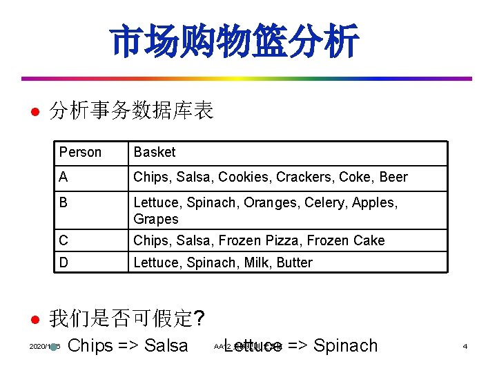
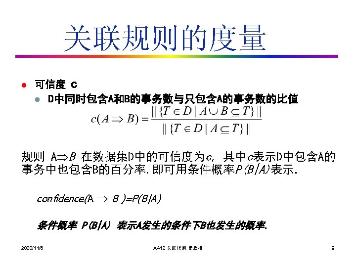
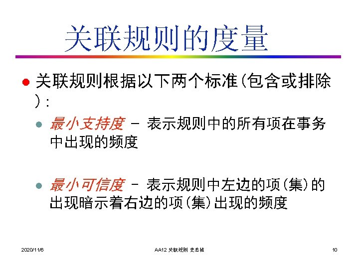
市场购物篮分析 l l 分析事务数据库表 Person Basket A Chips, Salsa, Cookies, Crackers, Coke, Beer B Lettuce, Spinach, Oranges, Celery, Apples, Grapes C Chips, Salsa, Frozen Pizza, Frozen Cake D Lettuce, Spinach, Milk, Butter 我们是否可假定? l 2020/11/6 Chips => Salsa Lettuce => Spinach AA 12 关联规则 史忠植 4

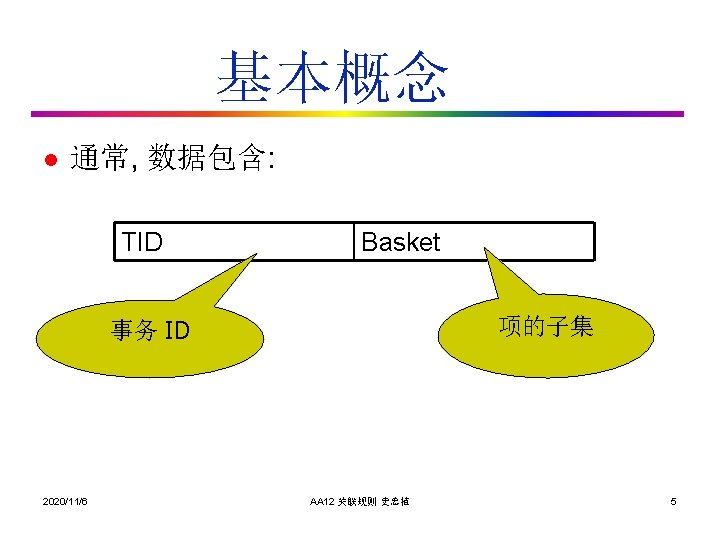
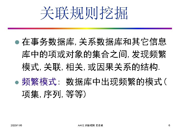
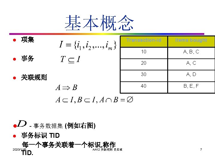
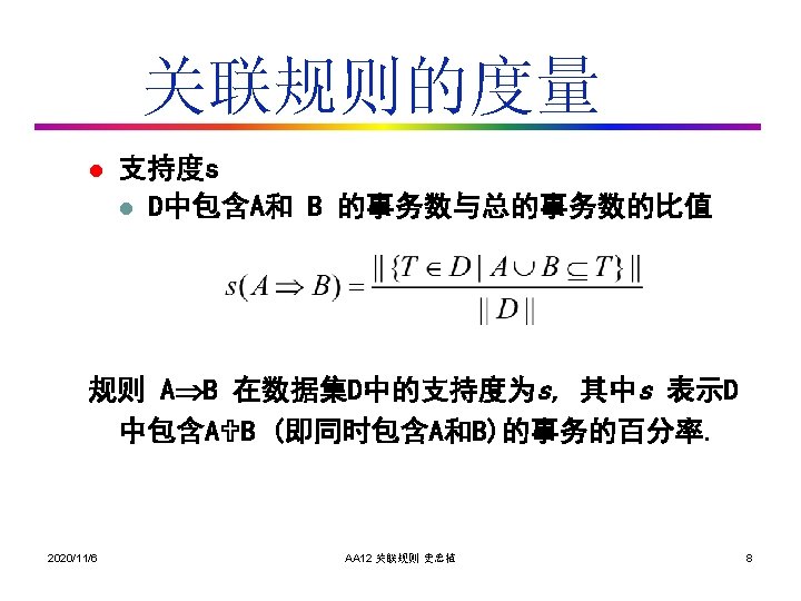
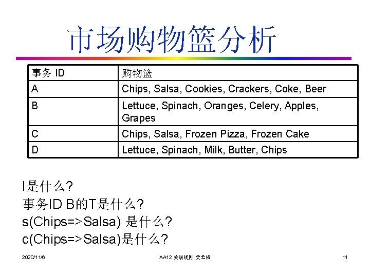
市场购物篮分析 事务 ID 购物篮 A Chips, Salsa, Cookies, Crackers, Coke, Beer B Lettuce, Spinach, Oranges, Celery, Apples, Grapes C Chips, Salsa, Frozen Pizza, Frozen Cake D Lettuce, Spinach, Milk, Butter, Chips I是什么? 事务ID B的T是什么? s(Chips=>Salsa) 是什么? c(Chips=>Salsa)是什么? 2020/11/6 AA 12 关联规则 史忠植 11

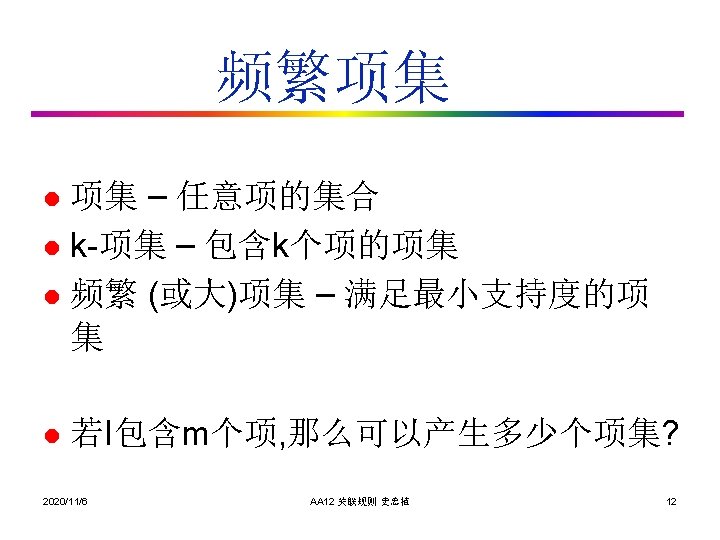
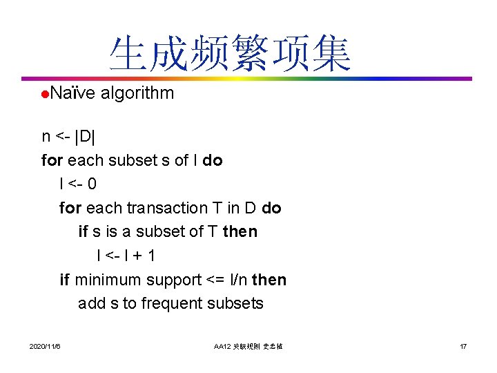
生成频繁项集 l. Naïve algorithm n <- |D| for each subset s of I do l <- 0 for each transaction T in D do if s is a subset of T then l <- l + 1 if minimum support <= l/n then add s to frequent subsets 2020/11/6 AA 12 关联规则 史忠植 17

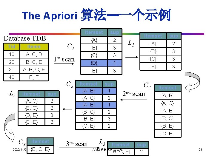
The Apriori 算法—一个示例 Database TDB Tid Items 10 A, C, D 20 B, C, E 30 A, B, C, E 40 B, E L 2 Itemset {A, C} {B, E} {C, E} Itemset sup {A} 2 {B} 3 {C} 3 {D} 1 {E} 3 C 1 1 st scan C 2 sup 2 2 3 2 Itemset {A, B} {A, C} {A, E} {B, C} {B, E} {C, E} sup 1 2 3 2 L 1 Itemset sup {A} 2 {B} 3 {C} 3 {E} 3 C 2 2 nd scan Itemset {A, B} {A, C} {A, E} {B, C} {B, E} {C, E} C 3 2020/11/6 Itemset {B, C, E} 3 rd scan L 3 Itemset AA 12 关联规则 史忠植 {B, C, E} sup 2 23

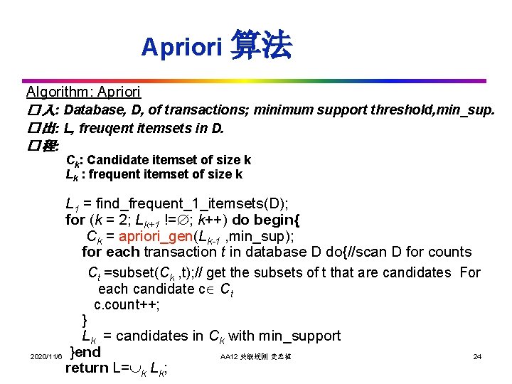
Apriori 算法 Algorithm: Apriori � 入: Database, D, of transactions; minimum support threshold, min_sup. � 出: L, freuqent itemsets in D. � 程: Ck: Candidate itemset of size k Lk : frequent itemset of size k L 1 = find_frequent_1_itemsets(D); for (k = 2; Lk+1 != ; k++) do begin{ Ck = apriori_gen(Lk-1 , min_sup); for each transaction t in database D do{//scan D for counts Ct =subset(Ck , t); // get the subsets of t that are candidates For each candidate c Ct c. count++; } Lk = candidates in Ck with min_support 2020/11/6 }end AA 12 关联规则 史忠植 24 return L= k Lk;

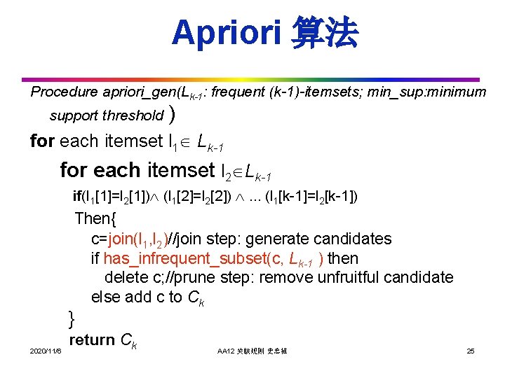
Apriori 算法 Procedure apriori_gen(Lk-1: frequent (k-1)-itemsets; min_sup: minimum support threshold ) for each itemset l 1 Lk-1 for each itemset l 2 Lk-1 if(l 1[1]=l 2[1]) (l 1[2]=l 2[2]) … (l 1[k-1]=l 2[k-1]) Then{ c=join(l 1, l 2)//join step: generate candidates if has_infrequent_subset(c, Lk-1 ) then delete c; //prune step: remove unfruitful candidate else add c to Ck } 2020/11/6 return Ck AA 12 关联规则 史忠植 25

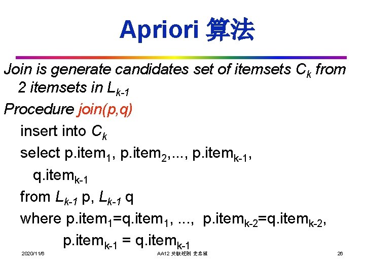
Apriori 算法 Join is generate candidates set of itemsets Ck from 2 itemsets in Lk-1 Procedure join(p, q) insert into Ck select p. item 1, p. item 2, . . . , p. itemk-1, q. itemk-1 from Lk-1 p, Lk-1 q where p. item 1=q. item 1, . . . , p. itemk-2=q. itemk-2, p. itemk-1 = q. itemk-1 2020/11/6 AA 12 关联规则 史忠植 26

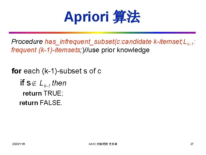
Apriori 算法 Procedure has_infrequent_subset(c: candidate k-itemset; Lk-1: frequent (k-1)-itemsets; )//use prior knowledge for each (k-1)-subset s of c if s Lk-1 then return TRUE; return FALSE. 2020/11/6 AA 12 关联规则 史忠植 27

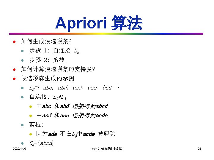
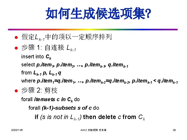
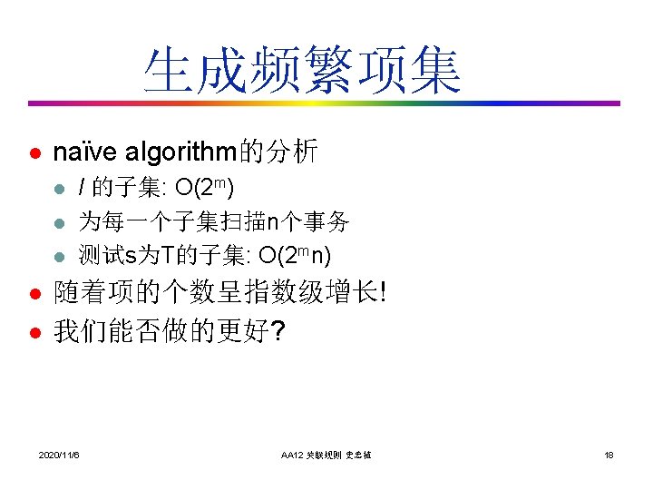
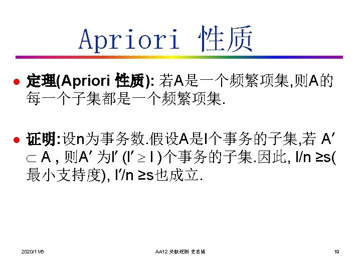
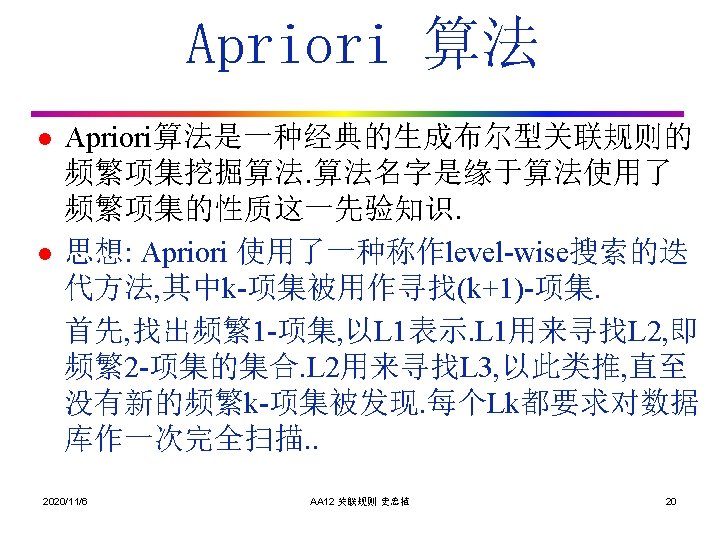
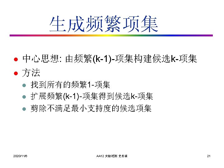
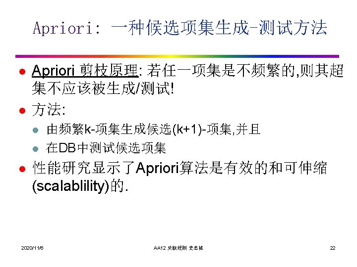
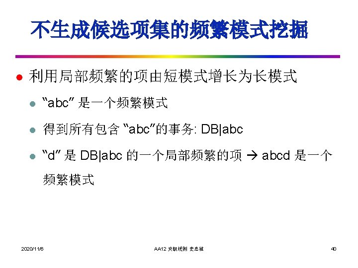
如何生成候选项集? l 假定Lk-1中的项以一定顺序排列 l 步骤 1: 自连接 Lk-1 insert into Ck select p. item 1, p. item 2, …, p. itemk-1, q. itemk-1 from Lk-1 p, Lk-1 q where p. item 1=q. item 1, …, p. itemk-2=q. itemk-2, p. itemk-1 < q. itemk-1 l 步骤 2: 剪枝 forall itemsets c in Ck do forall (k-1)-subsets s of c do if (s is not in Lk-1) then delete c from Ck 2020/11/6 AA 12 关联规则 史忠植 29

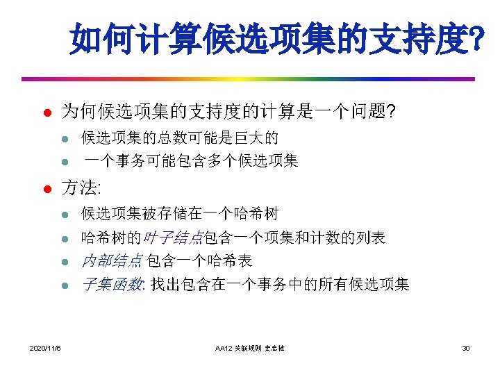
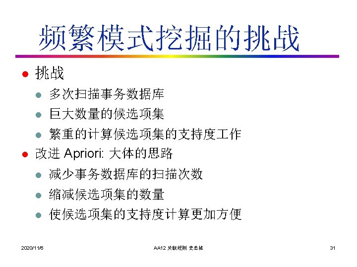
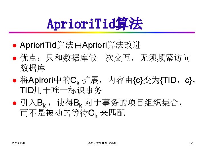
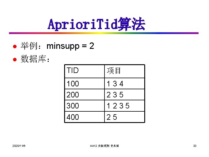
Apriori. Tid算法 l l 举例：minsupp = 2 数据库： 2020/11/6 TID 项目 100 200 300 400 134 235 1235 25 AA 12 关联规则 史忠植 33

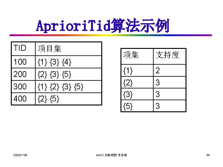
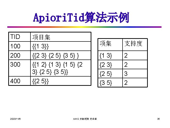
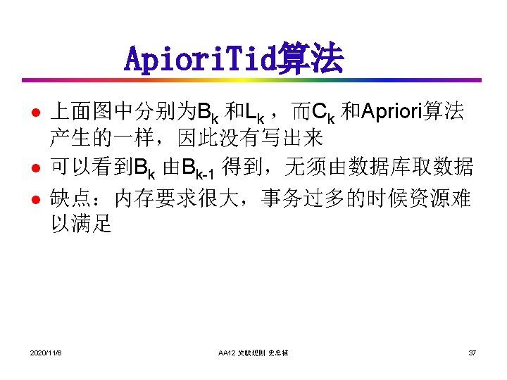
Apiori. Tid算法示例 TID 100 200 300 400 2020/11/6 项目集 {{1 3}} {{2 3} {2 5} {3 5} } {{1 2} {1 3} {1 5} {2 3} {2 5} {3 5}} {{2 5}} AA 12 关联规则 史忠植 项集 支持度 {1 3} {2 5} {3 5} 2 2 35

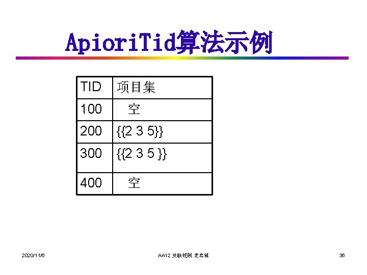
Apiori. Tid算法示例 TID 项目集 100 空 200 {{2 3 5}} 300 {{2 3 5 }} 400 2020/11/6 空 AA 12 关联规则 史忠植 36

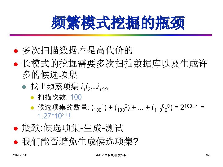
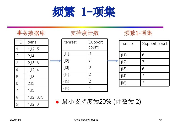
频繁 1 -项集 事务数据库 支持度计数 频繁1 -项集 TID Items 1 I 1, I 2, I 5 2 I 2, I 4 3 I 2, I 3, I 6 4 I 1, I 2, I 4 5 I 1, I 3 6 I 2, I 3 7 I 1, I 3 8 I 1, I 2, I 3, I 5 9 I 1, I 2, I 3 2020/11/6 l Itemset Support count {I 1} 6 {I 2} 7 {I 3} 6 {I 4} 2 {I 5} 2 {I 6} 1 最小支持度为 20% (计数为 2) AA 12 关联规则 史忠植 43

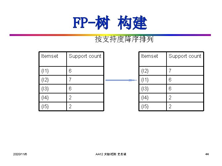
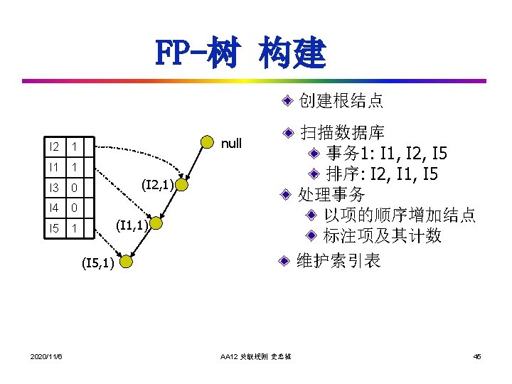
FP-树 构建 按支持度降序排列 2020/11/6 Itemset Support count {I 1} 6 {I 2} 7 {I 1} 6 {I 3} 6 {I 4} 2 {I 5} 2 AA 12 关联规则 史忠植 44

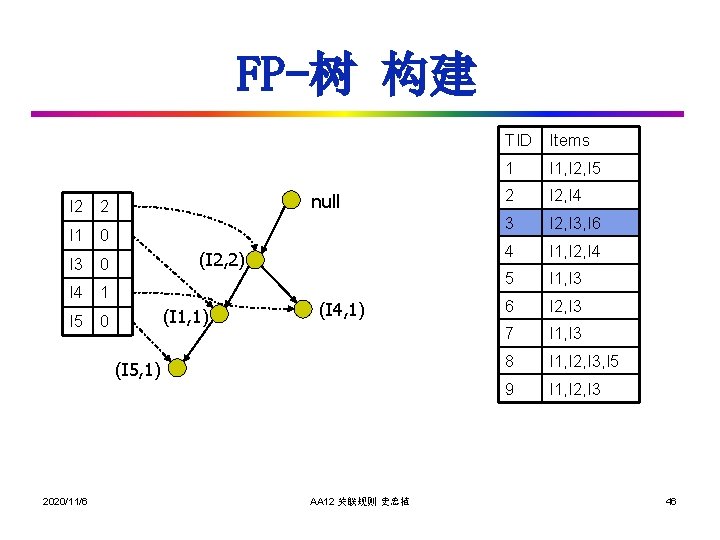
FP-树 构建 TID Items null I 2 2 I 1 0 (I 2, 2) I 3 0 I 4 1 (I 1, 1) I 5 0 (I 4, 1) (I 5, 1) 2020/11/6 AA 12 关联规则 史忠植 1 I 1, I 2, I 5 2 I 2, I 4 3 I 2, I 3, I 6 4 I 1, I 2, I 4 5 I 1, I 3 6 I 2, I 3 7 I 1, I 3 8 I 1, I 2, I 3, I 5 9 I 1, I 2, I 3 46

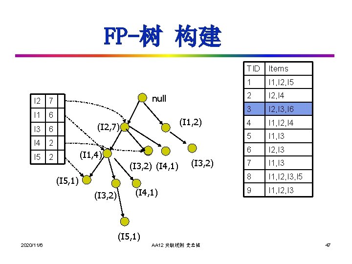
FP-树 构建 TID Items null I 2 7 I 1 6 (I 1, 2) (I 2, 7) I 3 6 I 4 2 (I 1, 4) I 5 2 (I 3, 2) (I 4, 1) (I 3, 2) (I 5, 1) (I 3, 2) (I 4, 1) 1 I 1, I 2, I 5 2 I 2, I 4 3 I 2, I 3, I 6 4 I 1, I 2, I 4 5 I 1, I 3 6 I 2, I 3 7 I 1, I 3 8 I 1, I 2, I 3, I 5 9 I 1, I 2, I 3 (I 5, 1) 2020/11/6 AA 12 关联规则 史忠植 47

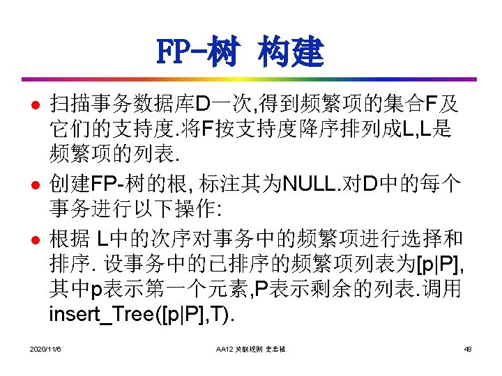
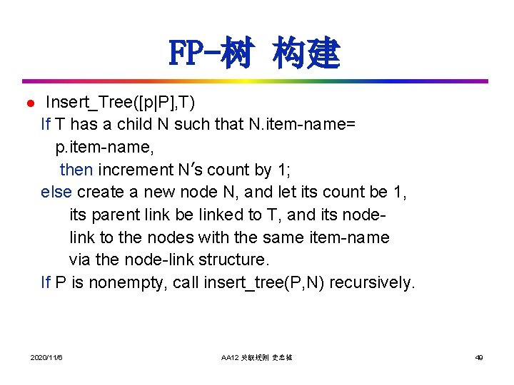
FP-树 构建 l Insert_Tree([p|P], T) If T has a child N such that N. item-name= p. item-name, then increment N’s count by 1; else create a new node N, and let its count be 1, its parent link be linked to T, and its nodelink to the nodes with the same item-name via the node-link structure. If P is nonempty, call insert_tree(P, N) recursively. 2020/11/6 AA 12 关联规则 史忠植 49

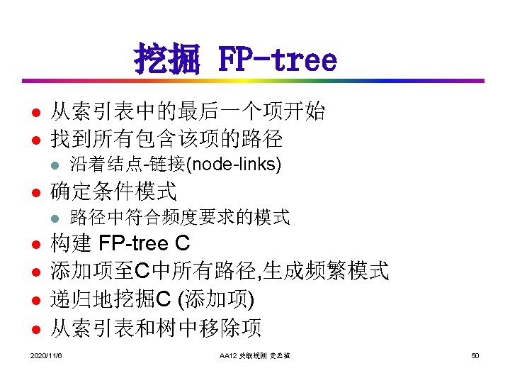
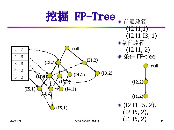
挖掘 FP-Tree null I 2 7 I 1 6 (I 1, 2) (I 2, 7) I 3 6 null I 4 2 (I 4, 1) (I 1, 4) I 5 2 (I 3, 2) (I 5, 1) (I 3, 2) (I 2, 2) (I 4, 1) (I 1, 2) (I 5, 1) 2020/11/6 前缀路径 (I 2 I 1, 1) (I 2 I 1 I 3, 1) 条件路径 (I 2 I 1, 2) 条件 FP-tree AA 12 关联规则 史忠植 (I 2 I 1 I 5, 2), (I 2 I 5, 2), (I 1 I 5, 2) 51

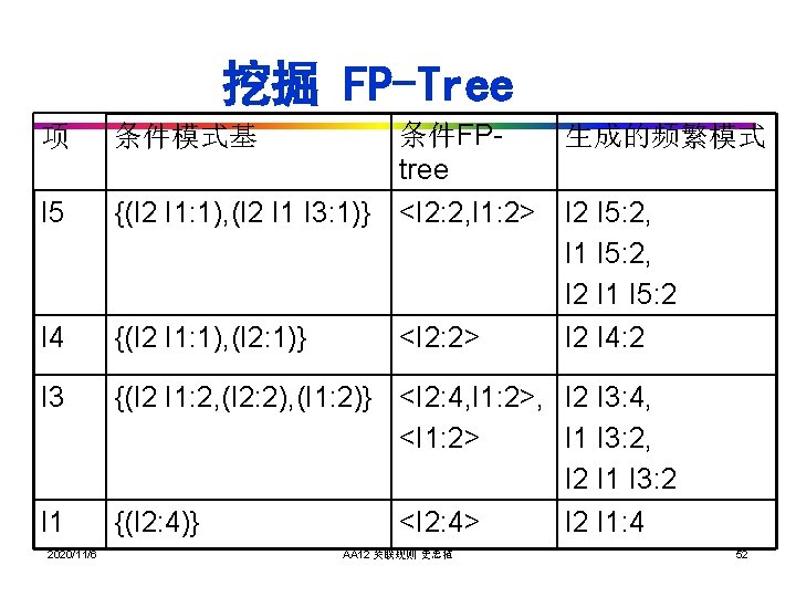
挖掘 FP-Tree 项 I 5 I 4 I 3 I 1 2020/11/6 条件FP生成的频繁模式 tree {(I 2 I 1: 1), (I 2 I 1 I 3: 1)} <I 2: 2, I 1: 2> I 2 I 5: 2, I 1 I 5: 2, I 2 I 1 I 5: 2 {(I 2 I 1: 1), (I 2: 1)} <I 2: 2> I 2 I 4: 2 条件模式基 {(I 2 I 1: 2, (I 2: 2), (I 1: 2)} <I 2: 4, I 1: 2>, I 2 I 3: 4, <I 1: 2> I 1 I 3: 2, I 2 I 1 I 3: 2 {(I 2: 4)} <I 2: 4> I 2 I 1: 4 AA 12 关联规则 史忠植 52

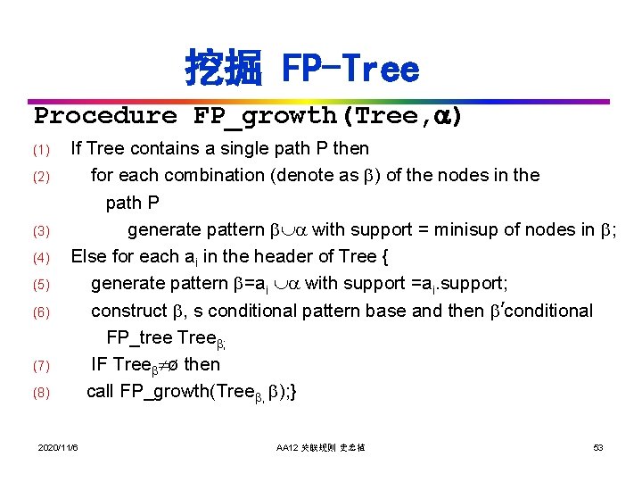
挖掘 FP-Tree Procedure FP_growth(Tree, ) (1) (2) (3) (4) (5) (6) (7) (8) If Tree contains a single path P then for each combination (denote as ) of the nodes in the path P generate pattern with support = minisup of nodes in ; Else for each ai in the header of Tree { generate pattern =ai with support =ai. support; construct , s conditional pattern base and then ’conditional FP_tree Tree ; IF Tree ø then call FP_growth(Tree , ); } 2020/11/6 AA 12 关联规则 史忠植 53

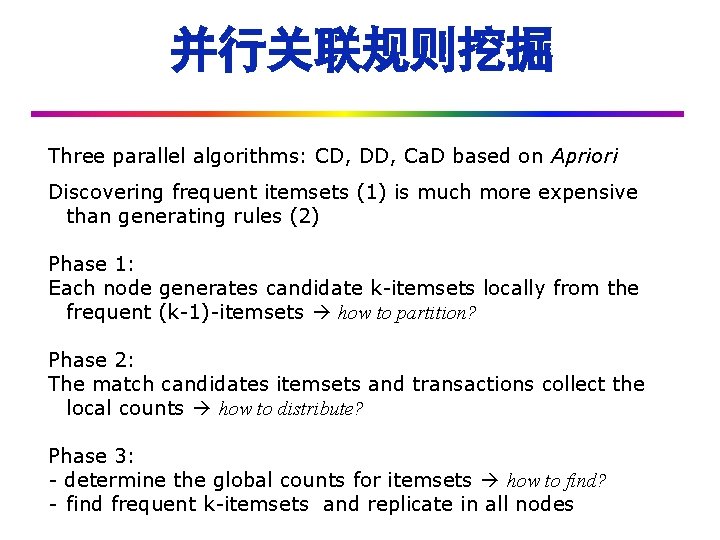
并行关联规则挖掘 Three parallel algorithms: CD, DD, Ca. D based on Apriori Discovering frequent itemsets (1) is much more expensive than generating rules (2) Phase 1: Each node generates candidate k-itemsets locally from the frequent (k-1)-itemsets how to partition? Phase 2: The match candidates itemsets and transactions collect the local counts how to distribute? Phase 3: - determine the global counts for itemsets how to find? - find frequent k-itemsets and replicate in all nodes

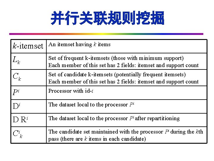
并行关联规则挖掘 k-itemset An itemset having k items Lk Set of frequent k-itemsets (those with minimum support) Each member of this set has 2 fields: itemset and support count Ck Set of candidate k-itemsets (potentially frequent itemsets) Each member of this set has 2 fields: itemset and support count Pi Processor with id-i Di The dataset local to the processor Pi D Ri The dataset local to the processor Pi after repartitioning Ci The candidate set maintained with the processor Pi during the kth pass (there are k items in each candidate) k

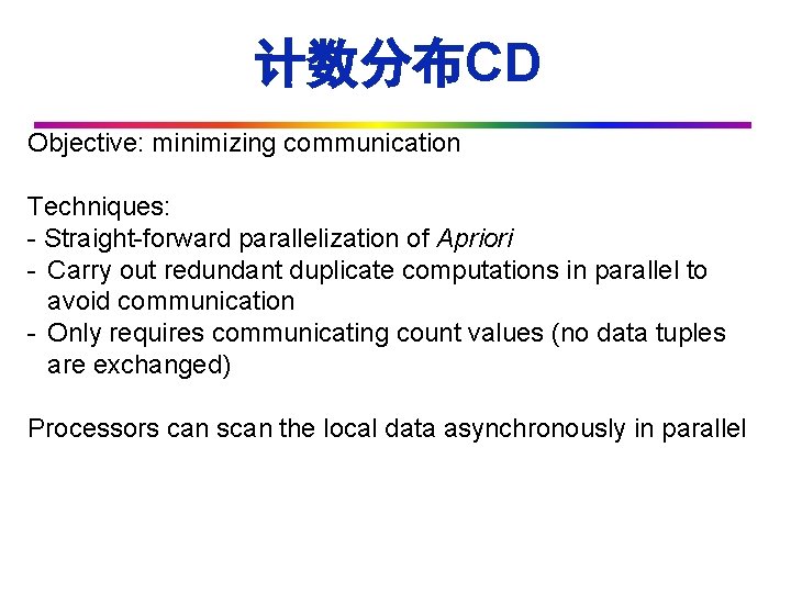
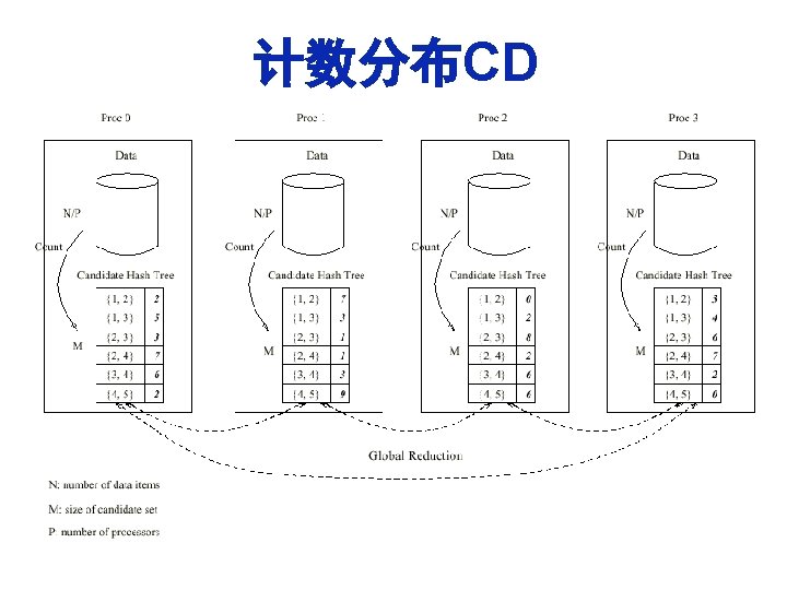
计数分布CD Objective: minimizing communication Techniques: - Straight-forward parallelization of Apriori - Carry out redundant duplicate computations in parallel to avoid communication - Only requires communicating count values (no data tuples are exchanged) Processors can scan the local data asynchronously in parallel

计数分布CD Algorithm: Pass 1: (1) Each processor Pi generates its local candidate itemset Ci 1 depending on the items present in its local data partition Di (2) Develop and Exchange local counts Ci 1 (3) Develop global support counts C 1

计数分布CD Algorithm: Pass k>1: (1) Pi generates the complete Ck using the complete Lk-1 created at the end of pass (k-1). Each processor has the identical Lk-1 thus generates identical Ck and puts its count values in a common order into a count array (2) Pi makes a pass over data partition Di and develop local support counts for candidates in Ck (3) Pi exchanges local Ck counts with all other processors to develop global Ck counts. All processors must synchronize. (4) Pi computes Lk from Ck (5) Pi independently decide to terminate or continue to the next pass

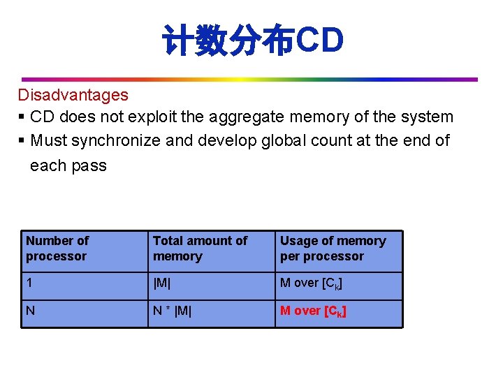
计数分布CD Disadvantages: § CD does not exploit the aggregate memory of the system § Must synchronize and develop global count at the end of each pass Number of processor Total amount of memory Usage of memory per processor 1 |M| M over [Ck] N N * |M| M over [Ck]

数据分布DD Objective: utilize aggregate main memory of the system effectively Technique: • Partitions the candidates into disjoint sets, which are assigned to different processors. Each processor works with the entire dataset but only portion of the candidate set. • Each processor counts mutually exclusive candidates. On a N-processor configuration, DD can count in a single pass candidate set that would require N pass in CD

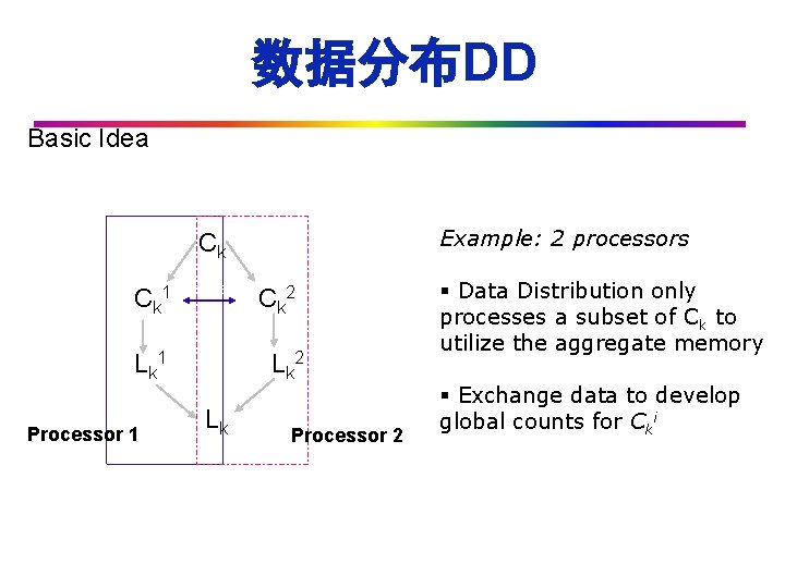
数据分布DD Basic Idea Example: 2 processors Ck C k 1 data L k 1 Processor 1 C k 2 Lk Processor 2 § Data Distribution only processes a subset of Ck to utilize the aggregate memory § Exchange data to develop global counts for Cki

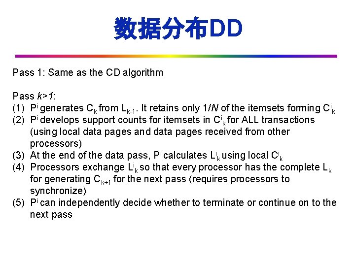
数据分布DD Algorithm: Pass 1: Same as the CD algorithm Pass k>1: (1) Pi generates Ck from Lk-1. It retains only 1/N of the itemsets forming Cik (2) Pi develops support counts for itemsets in Cik for ALL transactions (using local data pages and data pages received from other processors) (3) At the end of the data pass, Pi calculates Lik using local Cik (4) Processors exchange Lik so that every processor has the complete Lk for generating Ck+1 for the next pass (requires processors to synchronize) (5) Pi can independently decide whether to terminate or continue on to the next pass

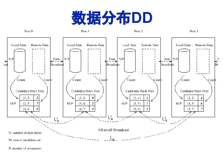
数据分布DD Li k Lk Li k

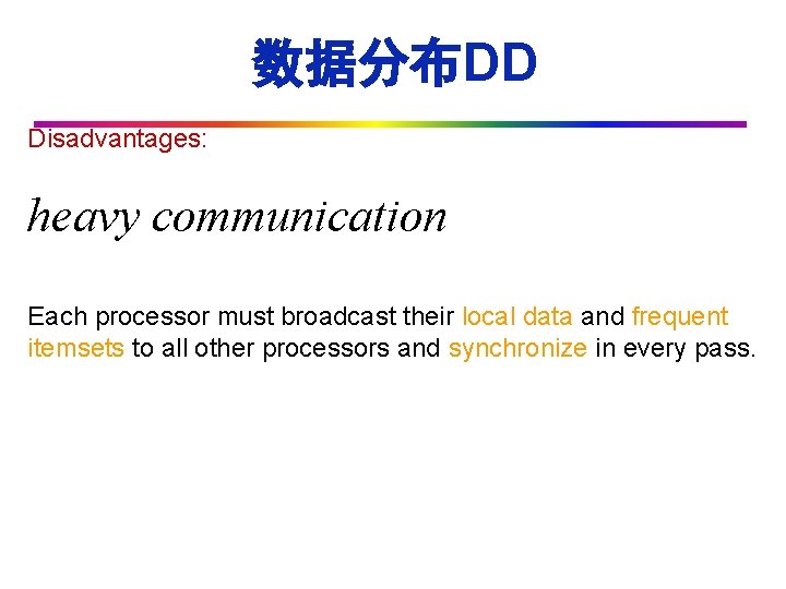
数据分布DD Disadvantages: heavy communication Each processor must broadcast their local data and frequent itemsets to all other processors and synchronize in every pass.

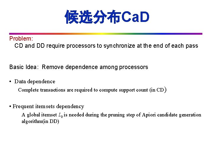
候选分布Ca. D Problem: CD and DD require processors to synchronize at the end of each pass Basic Idea: Remove dependence among processors • Data dependence Complete transactions are required to compute support count (in CD) • Frequent itemsets dependency A global itemset Lk is needed during the pruning step of Apiori candidate generation algorithm(in DD)

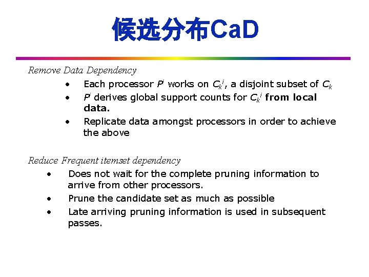
候选分布Ca. D Remove Data Dependency • • • Each processor Pi works on Cki, a disjoint subset of Ck Pi derives global support counts for Cki from local data. Replicate data amongst processors in order to achieve the above Reduce Frequent itemset dependency • • • Does not wait for the complete pruning information to arrive from other processors. Prune the candidate set as much as possible Late arriving pruning information is used in subsequent passes.

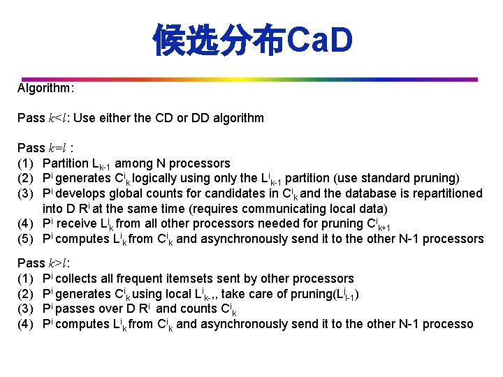
候选分布Ca. D Algorithm: Pass k<l: Use either the CD or DD algorithm Pass k=l : (1) Partition Lk-1 among N processors (2) Pi generates Cik logically using only the Lik-1 partition (use standard pruning) (3) Pi develops global counts for candidates in Cik and the database is repartitioned into D Ri at the same time (requires communicating local data) (4) Pi receive Ljk from all other processors needed for pruning Cik+1 (5) Pi computes Lik from Cik and asynchronously send it to the other N-1 processors Pass k>l: (1) Pi collects all frequent itemsets sent by other processors (2) Pi generates Cik using local Lik-, , take care of pruning(Ljl-1) (3) Pi passes over D Ri and counts Cik (4) Pi computes Lik from Cik and asynchronously send it to the other N-1 processors

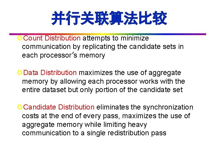
并行关联算法比较 µCount Distribution attempts to minimize communication by replicating the candidate sets in each processor’s memory µData Distribution maximizes the use of aggregate memory by allowing each processor works with the entire dataset but only portion of the candidate set µCandidate Distribution eliminates the synchronization costs at the end of every pass, maximizes the use of aggregate memory while limiting heavy communication to a single redistribution pass

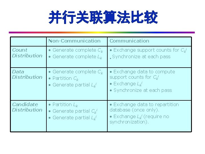
并行关联算法比较 Non-Communication Count Distribution • Generate complete Ck • Generate complete Lk • Exchange support counts for Cki • Synchronize at each pass Data Distribution • Generate complete Ck • Partition Ck • Generate partial Lki • Exchange data to compute support counts for Cki • Exchange Lki • Synchronize at each pass Candidate Distribution • Partition Lk • Generate partial Cki • Generate partial Lki • Exchange data to repartition database (once only). • Exchange Lki (require no synchronization).

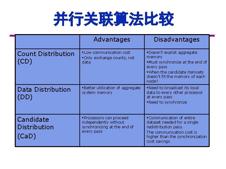
并行关联算法比较 Advantages Disadvantages Count Distribution (CD) §Low communication cost §Only exchange counts, not data §Doesn’t exploit aggregate memory §Must synchronize at the end of every pass §When the candidate itemsets doesn’t fit the memory of each node? Data Distribution (DD) §Better utilization of aggregate system memory §Need to broadcast its local data to every other processor at every pass §Need to synchronize Candidate Distribution (Ca. D) §Processors can proceed independently without synchronizing at the end of every pass §Communication of entire dataset needed for a single redistribution pass. The communication cost is higher than the synchronization cost savings

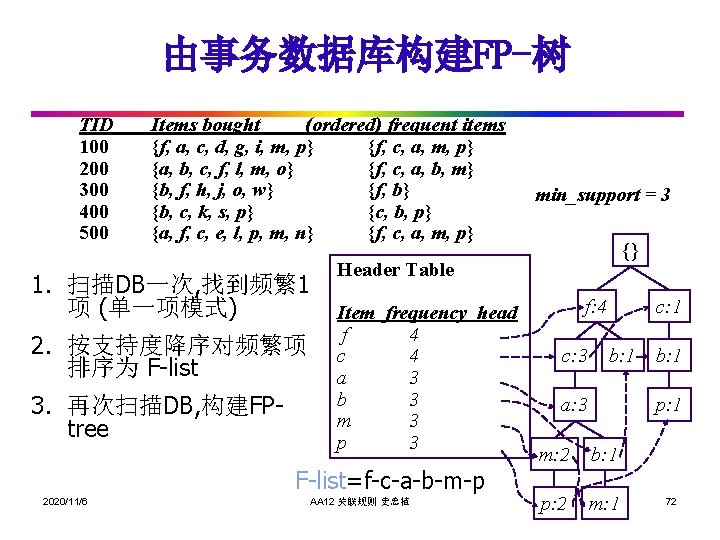
由事务数据库构建FP-树 TID 100 200 300 400 500 Items bought (ordered) frequent items {f, a, c, d, g, i, m, p} {f, c, a, m, p} {a, b, c, f, l, m, o} {f, c, a, b, m} {b, f, h, j, o, w} {f, b} {b, c, k, s, p} {c, b, p} {a, f, c, e, l, p, m, n} {f, c, a, m, p} 1. 扫描DB一次, 找到频繁1 项 (单一项模式) 2. 按支持度降序对频繁项 排序为 F-list 3. 再次扫描DB, 构建FPtree {} Header Table Item frequency head f 4 c 4 a 3 b 3 m 3 p 3 F-list=f-c-a-b-m-p 2020/11/6 min_support = 3 AA 12 关联规则 史忠植 f: 4 c: 3 c: 1 b: 1 a: 3 b: 1 p: 1 m: 2 b: 1 p: 2 m: 1 72

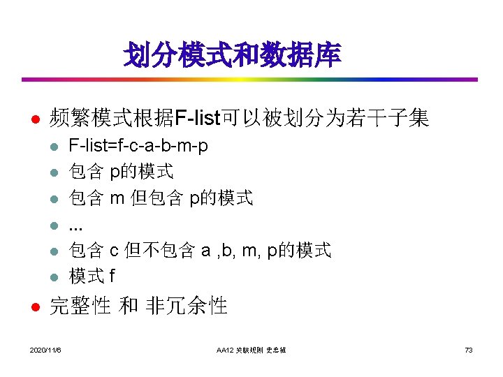
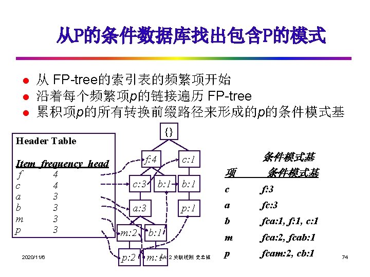
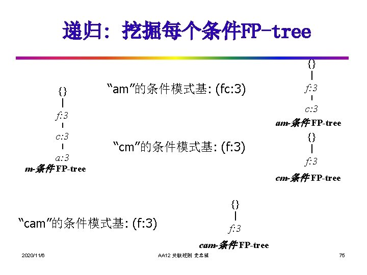
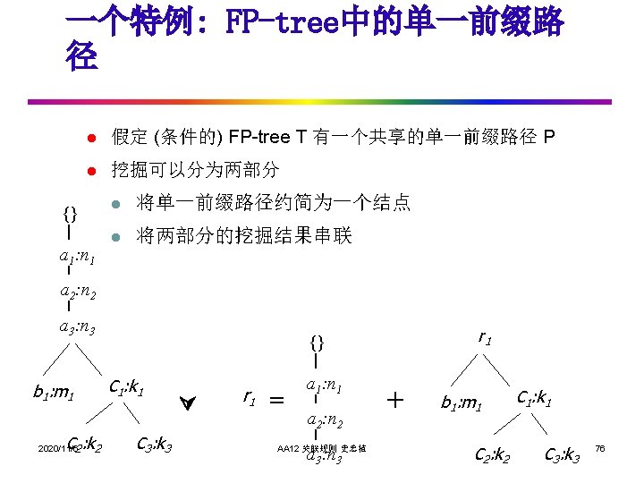
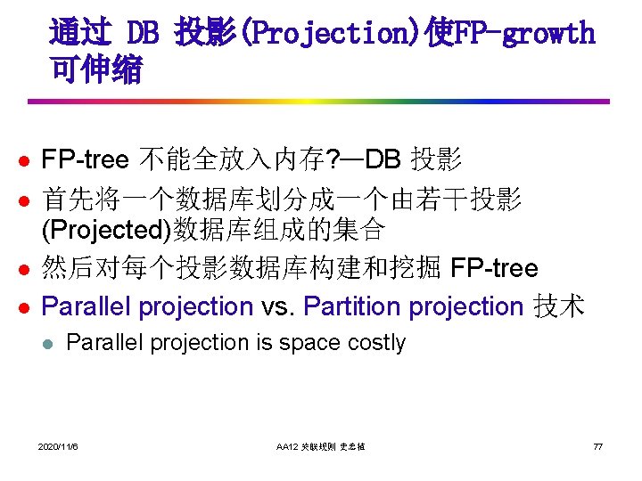
通过 DB 投影(Projection)使FP-growth 可伸缩 l l FP-tree 不能全放入内存? —DB 投影 首先将一个数据库划分成一个由若干投影 (Projected)数据库组成的集合 然后对每个投影数据库构建和挖掘 FP-tree Parallel projection vs. Partition projection 技术 l Parallel projection is space costly 2020/11/6 AA 12 关联规则 史忠植 77

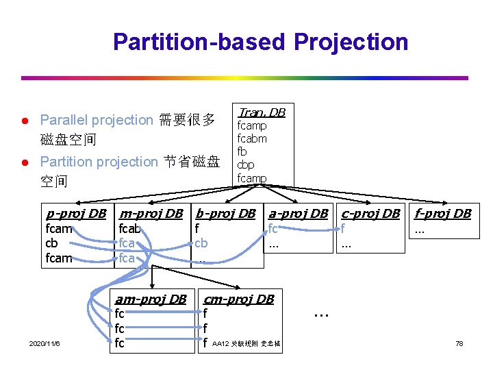
Partition-based Projection l l Parallel projection 需要很多 磁盘空间 Partition projection 节省磁盘 空间 p-proj DB fcam cb fcamp fcabm fb cbp fcamp m-proj DB b-proj DB fcab fca am-proj DB 2020/11/6 Tran. DB fc fc fc f cb … a-proj DB fc … cm-proj DB f f f AA 12 关联规则 史忠植 c-proj DB f … f-proj DB … … 78

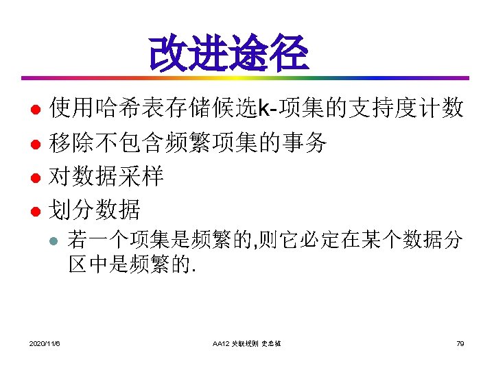
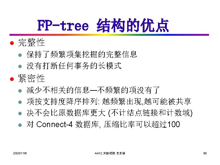
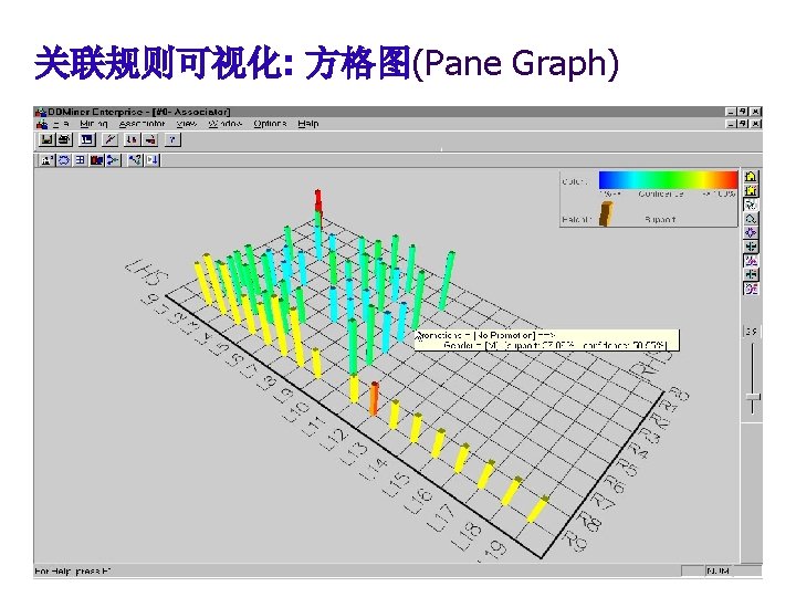
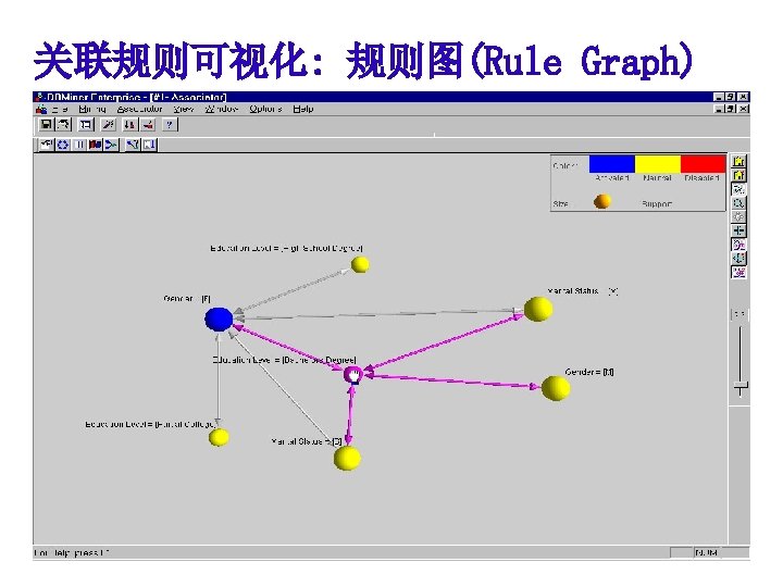
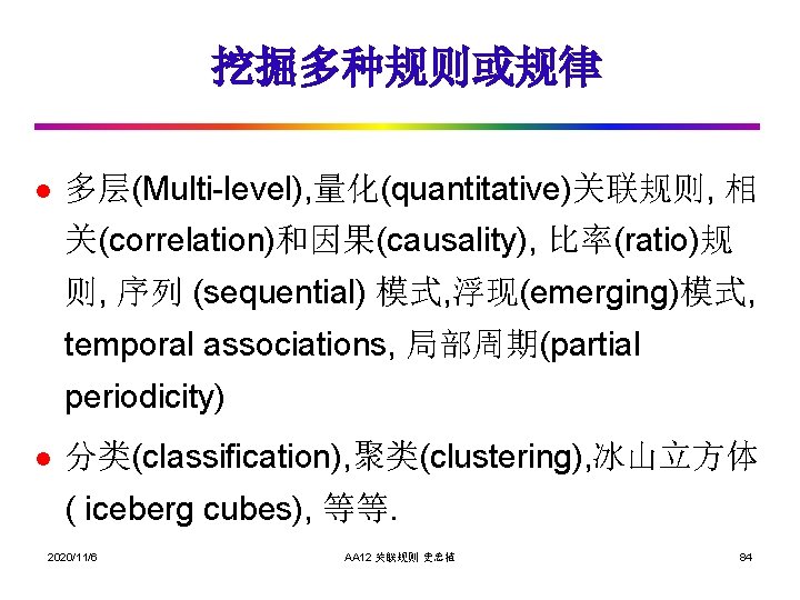
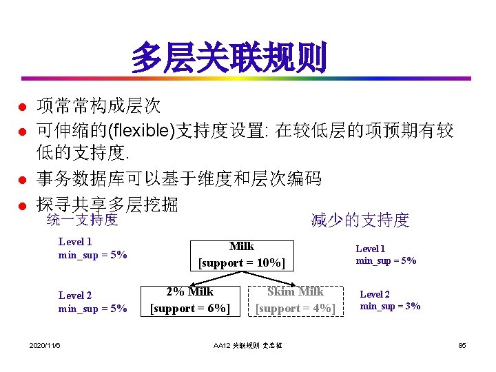
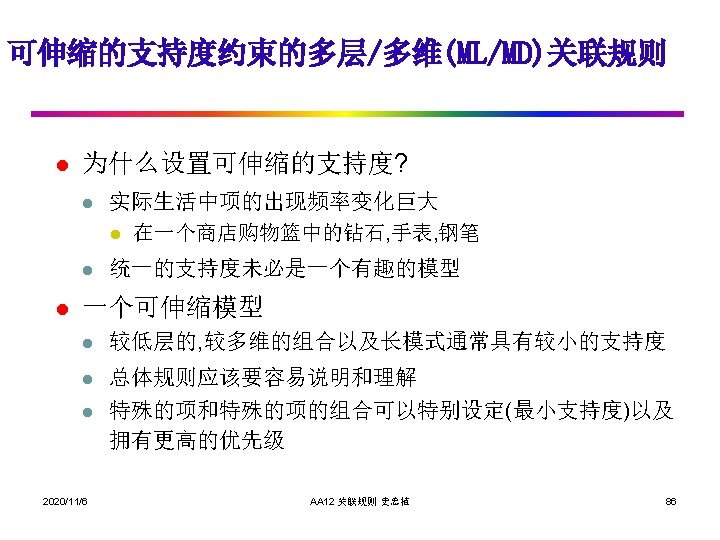
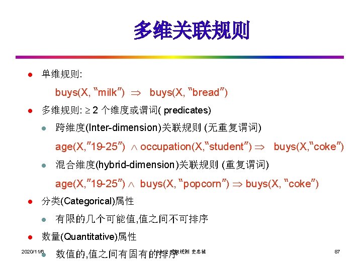
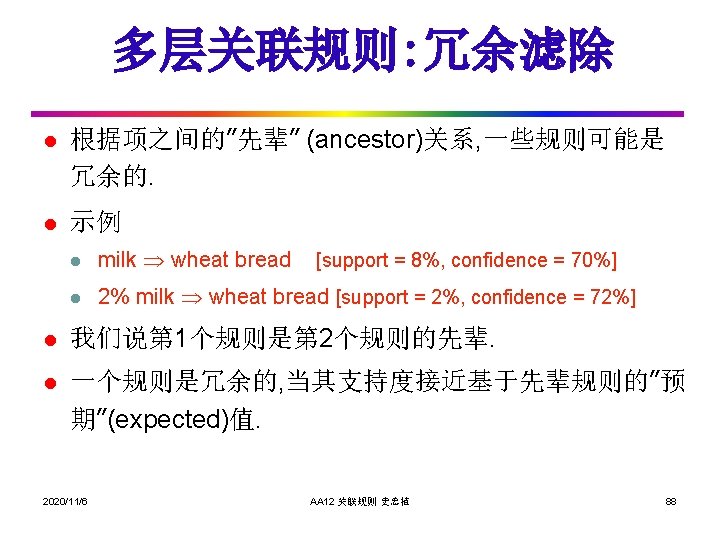
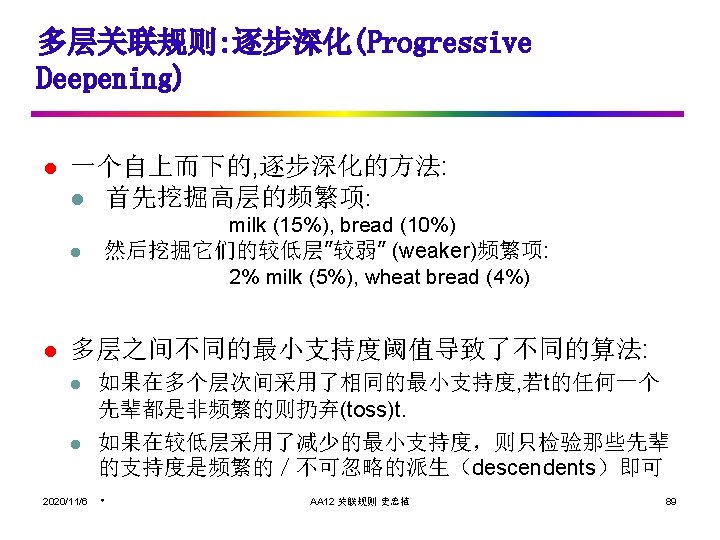
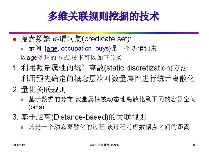
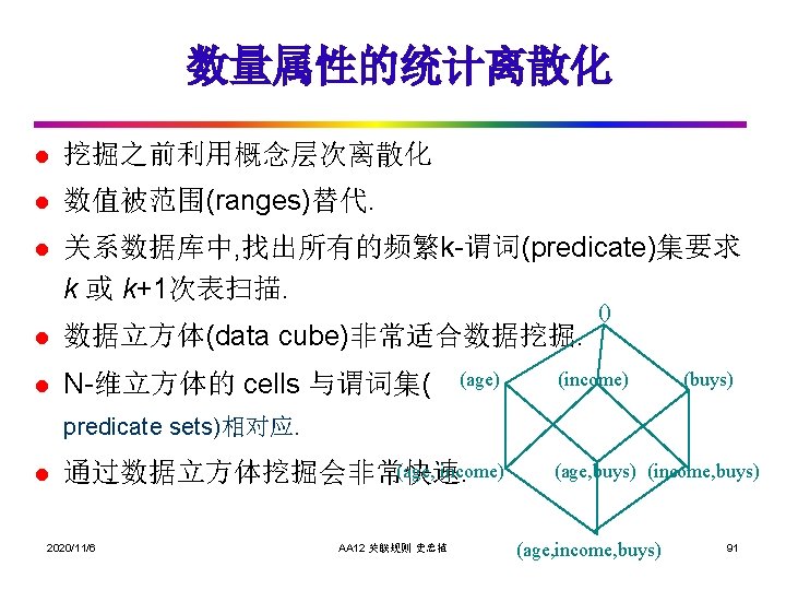
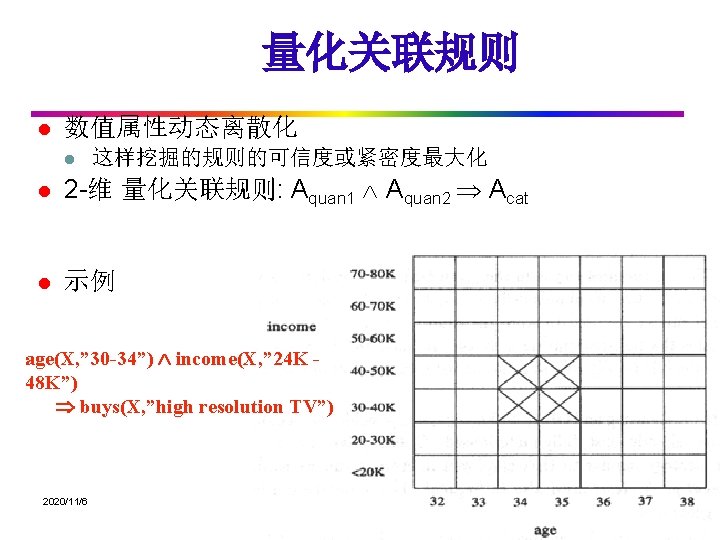
挖掘多种规则或规律 l 多层(Multi-level), 量化(quantitative)关联规则, 相 关(correlation)和因果(causality), 比率(ratio)规 则, 序列 (sequential) 模式, 浮现(emerging)模式, temporal associations, 局部周期(partial periodicity) l 分类(classification), 聚类(clustering), 冰山立方体 ( iceberg cubes), 等等. 2020/11/6 AA 12 关联规则 史忠植 84

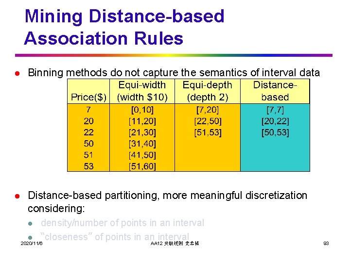
Mining Distance-based Association Rules l Binning methods do not capture the semantics of interval data l Distance-based partitioning, more meaningful discretization considering: l l density/number of points in an interval “closeness” of points in an interval 2020/11/6 AA 12 关联规则 史忠植 93

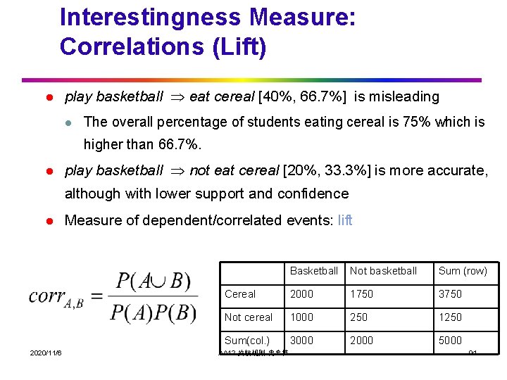
Interestingness Measure: Correlations (Lift) l play basketball eat cereal [40%, 66. 7%] is misleading l The overall percentage of students eating cereal is 75% which is higher than 66. 7%. l play basketball not eat cereal [20%, 33. 3%] is more accurate, although with lower support and confidence l 2020/11/6 Measure of dependent/correlated events: lift Basketball Not basketball Sum (row) Cereal 2000 1750 3750 Not cereal 1000 250 1250 Sum(col. ) 3000 2000 5000 AA 12 关联规则 史忠植 94

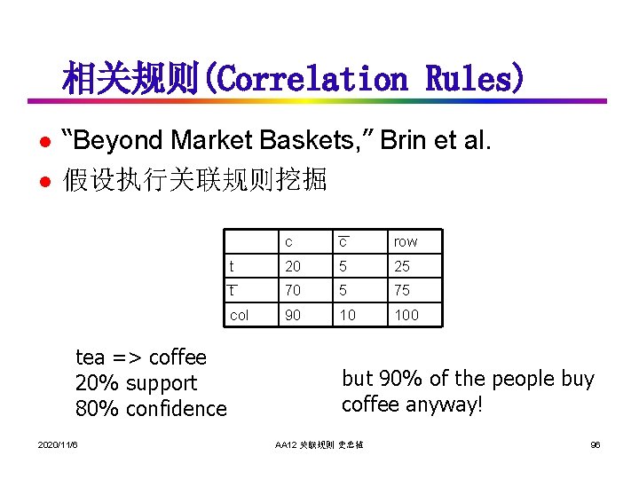
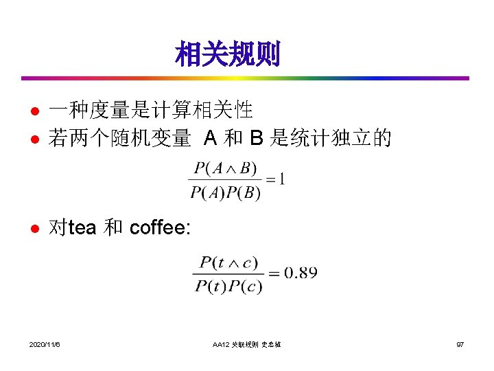
相关规则(Correlation Rules) l l “Beyond Market Baskets, ” Brin et al. 假设执行关联规则挖掘 tea => coffee 20% support 80% confidence 2020/11/6 c c row t 20 5 25 t 70 5 75 col 90 10 100 but 90% of the people buy coffee anyway! AA 12 关联规则 史忠植 96

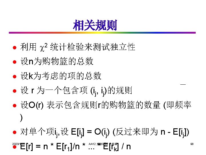
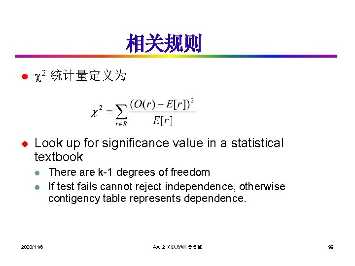
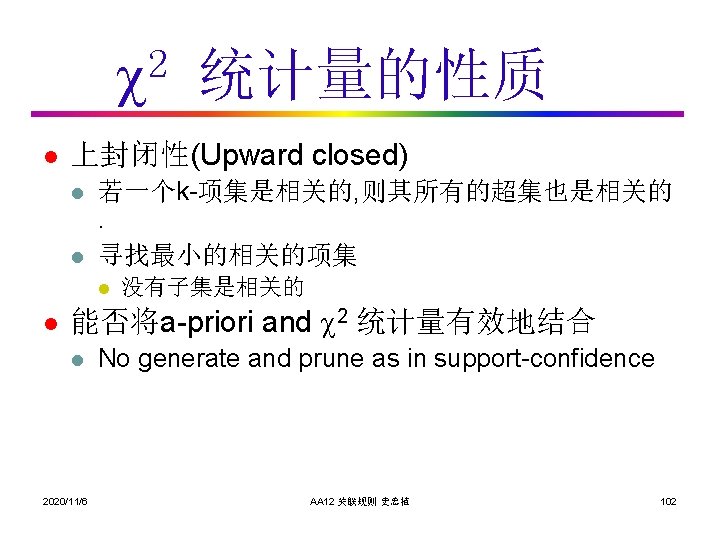
相关规则 l 2 统计量定义为 l Look up for significance value in a statistical textbook l l 2020/11/6 There are k-1 degrees of freedom If test fails cannot reject independence, otherwise contigency table represents dependence. AA 12 关联规则 史忠植 99

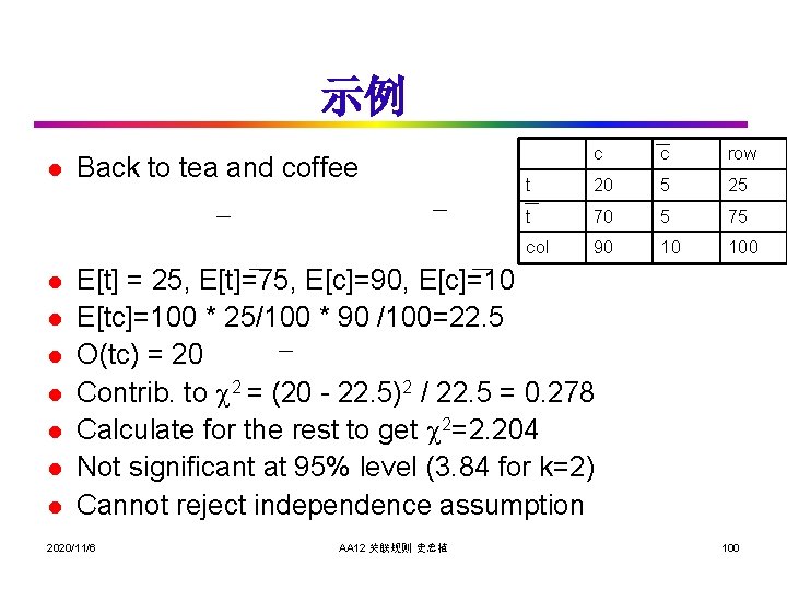
示例 l l l l Back to tea and coffee c c row t 20 5 25 t 70 5 75 col 90 10 100 E[t] = 25, E[t]=75, E[c]=90, E[c]=10 E[tc]=100 * 25/100 * 90 /100=22. 5 O(tc) = 20 Contrib. to 2 = (20 - 22. 5)2 / 22. 5 = 0. 278 Calculate for the rest to get 2=2. 204 Not significant at 95% level (3. 84 for k=2) Cannot reject independence assumption 2020/11/6 AA 12 关联规则 史忠植 100

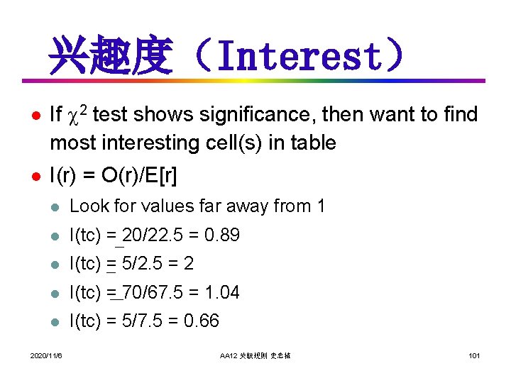
兴趣度（Interest） l l If 2 test shows significance, then want to find most interesting cell(s) in table I(r) = O(r)/E[r] l Look for values far away from 1 l I(tc) = 20/22. 5 = 0. 89 l I(tc) = 5/2. 5 = 2 l I(tc) = 70/67. 5 = 1. 04 l I(tc) = 5/7. 5 = 0. 66 2020/11/6 AA 12 关联规则 史忠植 101

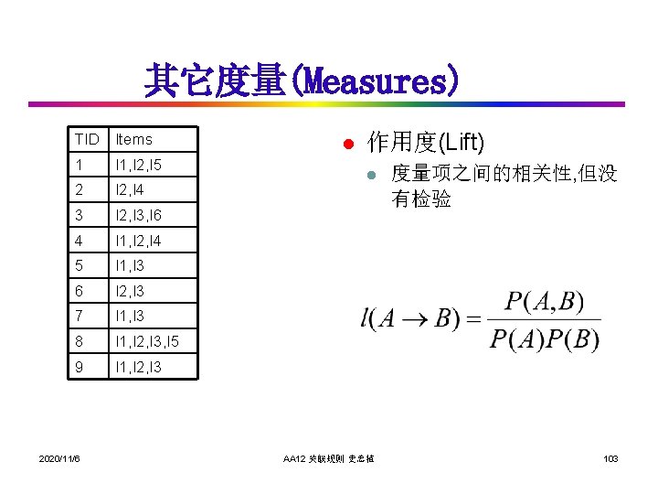
其它度量(Measures) TID Items 1 I 1, I 2, I 5 2 I 2, I 4 3 I 2, I 3, I 6 4 I 1, I 2, I 4 5 I 1, I 3 6 I 2, I 3 7 I 1, I 3 8 I 1, I 2, I 3, I 5 9 I 1, I 2, I 3 2020/11/6 l 作用度(Lift) l 度量项之间的相关性, 但没 有检验 AA 12 关联规则 史忠植 103

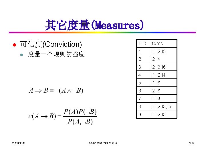
其它度量(Measures) l 可信度(Conviction) l 2020/11/6 TID Items 度量一个规则的强度 AA 12 关联规则 史忠植 1 I 1, I 2, I 5 2 I 2, I 4 3 I 2, I 3, I 6 4 I 1, I 2, I 4 5 I 1, I 3 6 I 2, I 3 7 I 1, I 3 8 I 1, I 2, I 3, I 5 9 I 1, I 2, I 3 104

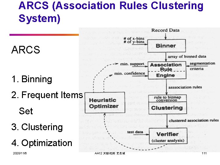
ARCS (Association Rules Clustering System) ARCS 1. Binning 2. Frequent Items Set 3. Clustering 4. Optimization 2020/11/6 AA 12 关联规则 史忠植 111

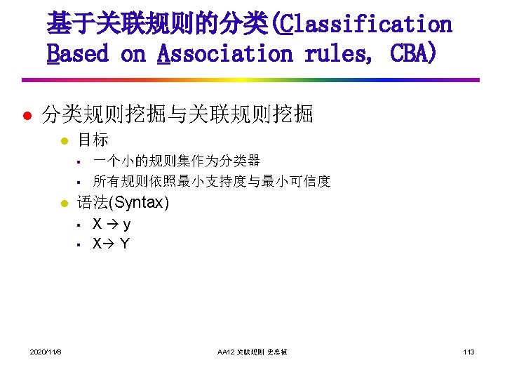
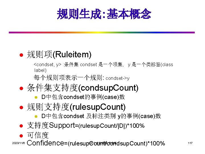
规则生成: 基本概念 l 规则项(Ruleitem) <condset, y> : 条件集 condset 是一个项集, y 是一个类标签(class label) 每个规则项表示一个规则: condset->y l 条件集支持度(condsup. Count) l l 规则支持度(rulesup. Count) l l l 2020/11/6 D中包含condset的事例(case)数 D中包含condset 及标注类别 y的事例(case)数 支持度Support=(rulesup. Count/|D|)*100% 可信度 Confidence=(rulesup. Count/condsup. Count)*100% AA 12 关联规则 史忠植 117

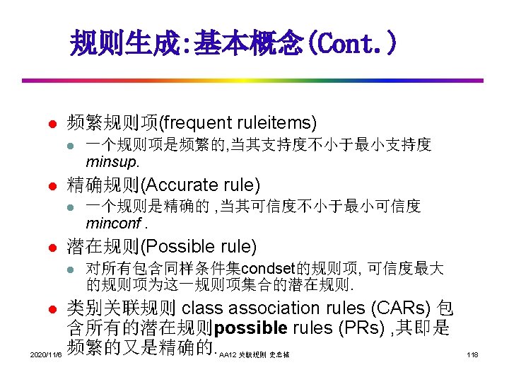
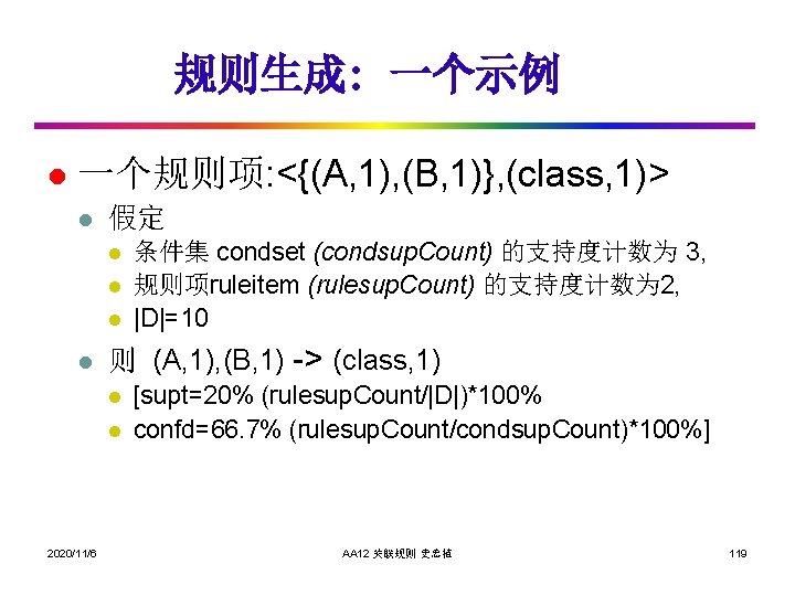
规则生成: 一个示例 l 一个规则项: <{(A, 1), (B, 1)}, (class, 1)> l 假定 l l 则 (A, 1), (B, 1) -> (class, 1) l l 2020/11/6 条件集 condset (condsup. Count) 的支持度计数为 3, 规则项ruleitem (rulesup. Count) 的支持度计数为 2, |D|=10 [supt=20% (rulesup. Count/|D|)*100% confd=66. 7% (rulesup. Count/condsup. Count)*100%] AA 12 关联规则 史忠植 119

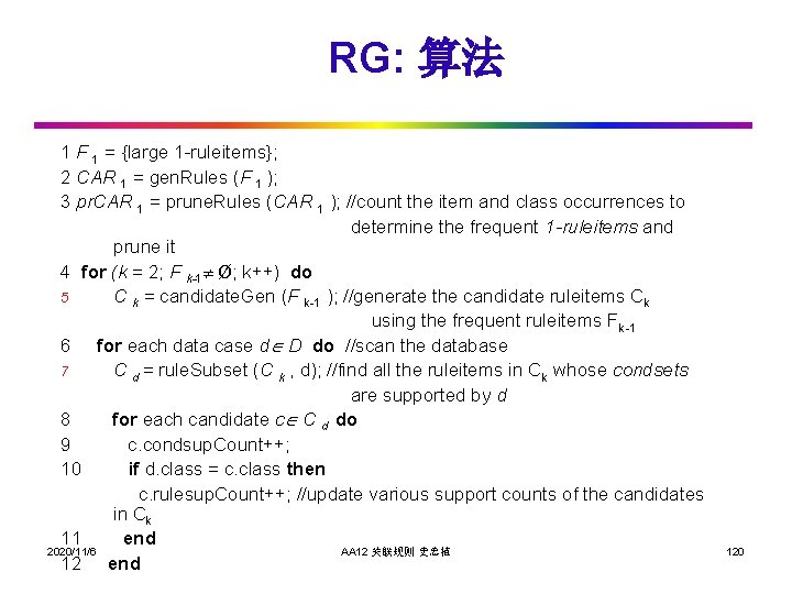
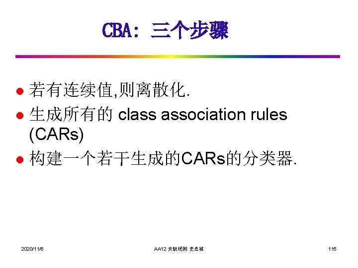
RG: 算法 1 F 1 = {large 1 -ruleitems}; 2 CAR 1 = gen. Rules (F 1 ); 3 pr. CAR 1 = prune. Rules (CAR 1 ); //count the item and class occurrences to determine the frequent 1 -ruleitems and prune it 4 for (k = 2; F k-1 Ø; k++) do 5 C k = candidate. Gen (F k-1 ); //generate the candidate ruleitems Ck using the frequent ruleitems F k-1 6 for each data case d D do //scan the database 7 C d = rule. Subset (C k , d); //find all the ruleitems in Ck whose condsets are supported by d 8 for each candidate c C d do 9 c. condsup. Count++; 10 if d. class = c. class then c. rulesup. Count++; //update various support counts of the candidates in Ck 11 end 2020/11/6 AA 12 关联规则 史忠植 12 end 120

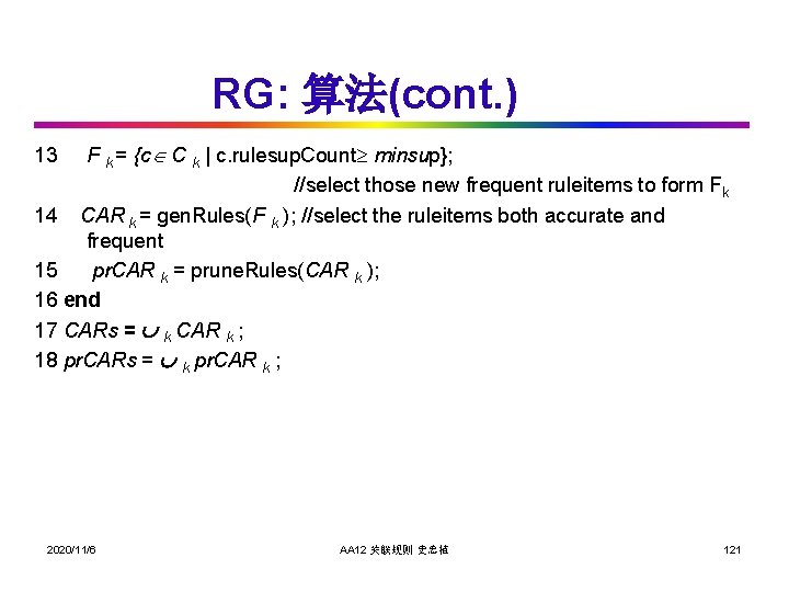
RG: 算法(cont. ) F k = {c C k | c. rulesup. Count minsup}; //select those new frequent ruleitems to form F k 14 CAR k = gen. Rules(F k ); //select the ruleitems both accurate and frequent 15 pr. CAR k = prune. Rules(CAR k ); 16 end 17 CARs = k CAR k ; 18 pr. CARs = k pr. CAR k ; 13 2020/11/6 AA 12 关联规则 史忠植 121

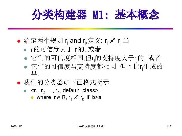
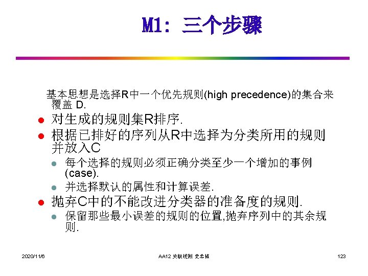
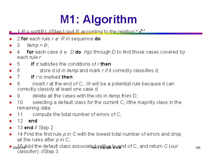
M 1: Algorithm 1 R = sort(R); //Step 1: sort R according to the relation “ ” l 2 for each rule r R in sequence do l 3 temp = Ø; l 4 for each case d D do //go through D to find those cases covered by each rule r l 5 if d satisfies the conditions of r then l 6 store d. id in temp and mark r if it correctly classifies d; l 7 if r is marked then l 8 insert r at the end of C; //r will be a potential rule because it can correctly classify at least one case d l 9 delete all the cases with the ids in temp from D; l 10 selecting a default class for the current C; //the majority class in the remaining data l 11 compute the total number of errors of C; l 12 end l 13 end // Step 2 l 14 Find the first rule p in C with the lowest total number of errors and drop all the rules after p in C; l 2020/11/6 15 Add the default class associated p to end of C, and return C (our AA 12 with 关联规则 史忠植 classifier). //Step 3 l 124

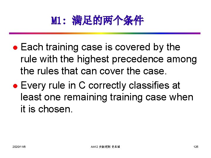
M 1: 满足的两个条件 Each training case is covered by the rule with the highest precedence among the rules that can cover the case. l Every rule in C correctly classifies at least one remaining training case when it is chosen. l 2020/11/6 AA 12 关联规则 史忠植 125

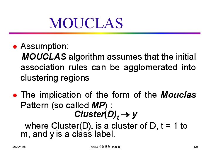
MOUCLAS l Assumption: MOUCLAS algorithm assumes that the initial association rules can be agglomerated into clustering regions l The implication of the form of the Mouclas Pattern (so called MP) : Cluster(D)t y where Cluster(D)t is a cluster of D, t = 1 to m, and y is a class label. 2020/11/6 AA 12 关联规则 史忠植 126

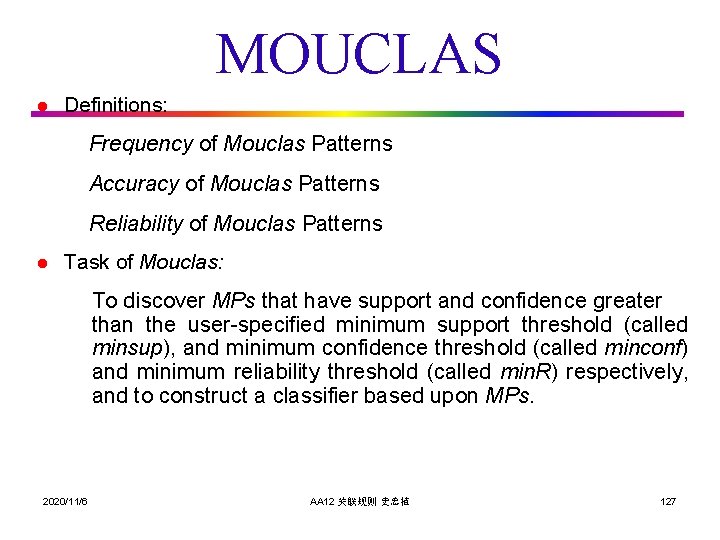
MOUCLAS l Definitions: Frequency of Mouclas Patterns Accuracy of Mouclas Patterns Reliability of Mouclas Patterns l Task of Mouclas: To discover MPs that have support and confidence greater than the user-specified minimum support threshold (called minsup), and minimum confidence threshold (called minconf) and minimum reliability threshold (called min. R) respectively, and to construct a classifier based upon MPs. 2020/11/6 AA 12 关联规则 史忠植 127

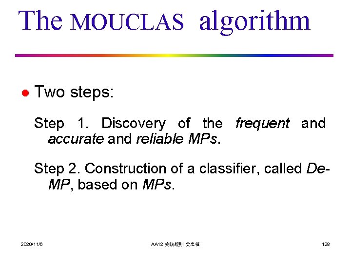
The MOUCLAS algorithm l Two steps: Step 1. Discovery of the frequent and accurate and reliable MPs. Step 2. Construction of a classifier, called De. MP, based on MPs. 2020/11/6 AA 12 关联规则 史忠植 128

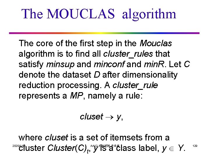
The MOUCLAS algorithm The core of the first step in the Mouclas algorithm is to find all cluster_rules that satisfy minsup and minconf and min. R. Let C denote the dataset D after dimensionality reduction processing. A cluster_rule represents a MP, namely a rule: cluset y, where cluset is a set of itemsets from a cluster Cluster(C)t, y is a class label, y Y. 2020/11/6 AA 12 关联规则 史忠植 129

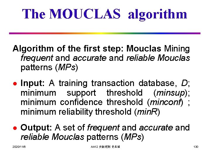
The MOUCLAS algorithm Algorithm of the first step: Mouclas Mining frequent and accurate and reliable Mouclas patterns (MPs) l Input: A training transaction database, D; minimum support threshold (minsup); minimum confidence threshold (minconf) ; minimum reliability threshold (min. R) l Output: A set of frequent and accurate and reliable Mouclas patterns (MPs) 2020/11/6 AA 12 关联规则 史忠植 130

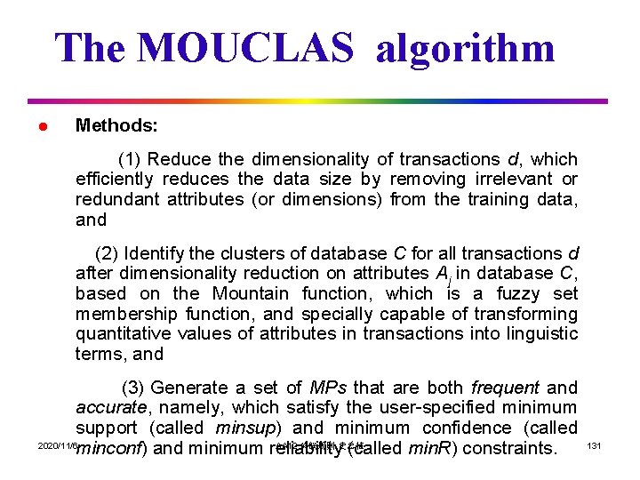
The MOUCLAS algorithm l Methods: (1) Reduce the dimensionality of transactions d, which efficiently reduces the data size by removing irrelevant or redundant attributes (or dimensions) from the training data, and (2) Identify the clusters of database C for all transactions d after dimensionality reduction on attributes Aj in database C, based on the Mountain function, which is a fuzzy set membership function, and specially capable of transforming quantitative values of attributes in transactions into linguistic terms, and (3) Generate a set of MPs that are both frequent and accurate, namely, which satisfy the user-specified minimum support (called minsup) and minimum confidence (called 2020/11/6 AA 12 关联规则 史忠植 minconf) and minimum reliability (called min. R) constraints. 131

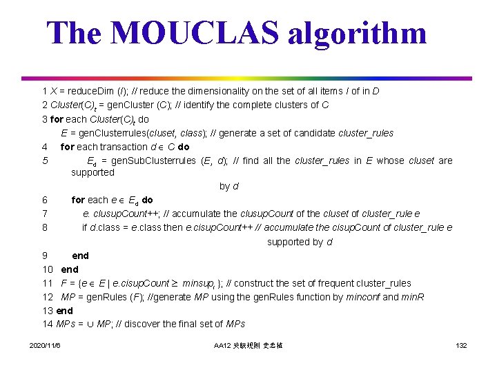
The MOUCLAS algorithm 1 X = reduce. Dim (I); // reduce the dimensionality on the set of all items I of in D 2 Cluster(C)t = gen. Cluster (C); // identify the complete clusters of C 3 for each Cluster(C)t do E = gen. Clusterrules(cluset, class); // generate a set of candidate cluster_rules 4 for each transaction d C do 5 Ed = gen. Sub. Clusterrules (E, d); // find all the cluster_rules in E whose cluset are supported by d 6 for each e Ed do 7 e. clusup. Count++; // accumulate the clusup. Count of the cluset of cluster_rule e 8 if d. class = e. class then e. cisup. Count++ // accumulate the cisup. Count of cluster_rule e supported by d 9 end 10 end 11 F = {e E e. cisup. Count minsupi }; // construct the set of frequent cluster_rules 12 MP = gen. Rules (F); //generate MP using the gen. Rules function by minconf and min. R 13 end 14 MPs = ∪ MP; // discover the final set of MPs 2020/11/6 AA 12 关联规则 史忠植 132

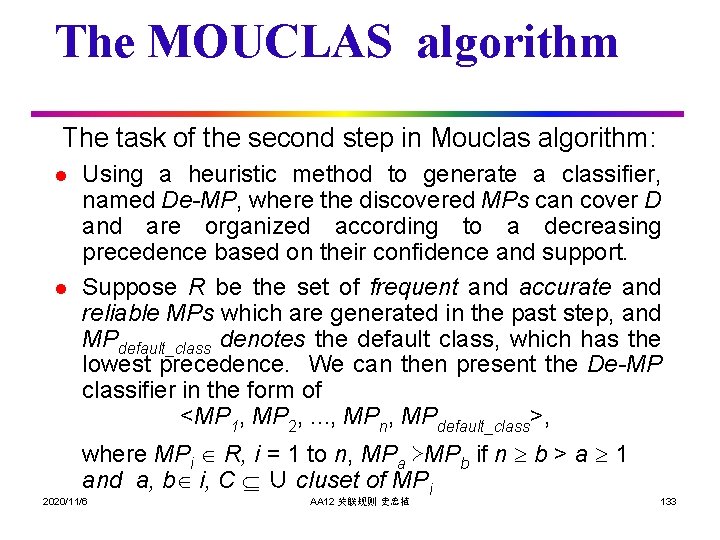
The MOUCLAS algorithm The task of the second step in Mouclas algorithm: l l Using a heuristic method to generate a classifier, named De-MP, where the discovered MPs can cover D and are organized according to a decreasing precedence based on their confidence and support. Suppose R be the set of frequent and accurate and reliable MPs which are generated in the past step, and MPdefault_class denotes the default class, which has the lowest precedence. We can then present the De-MP classifier in the form of <MP 1, MP 2, …, MPn, MPdefault_class>, where MPi R, i = 1 to n, MPa ≻MPb if n b > a 1 and a, b i, C ∪ cluset of MPi 2020/11/6 AA 12 关联规则 史忠植 133

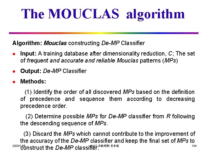
The MOUCLAS algorithm Algorithm: Mouclas constructing De-MP Classifier l Input: A training database after dimensionality reduction, C; The set of frequent and accurate and reliable Mouclas patterns (MPs) l Output: De-MP Classifier l Methods: (1) Identify the order of all discovered MPs based on the definition of precedence and sequence them according to decreasing precedence order. (2) Determine possible MPs for De-MP classifier from R following the descending sequence of MPs. (3) Discard the MPs which cannot contribute to the improvement of the accuracy of the De-MP classifier and keep the final set of MPs to 2020/11/6 AA 12 关联规则 史忠植 134 construct the De-MP classifier.

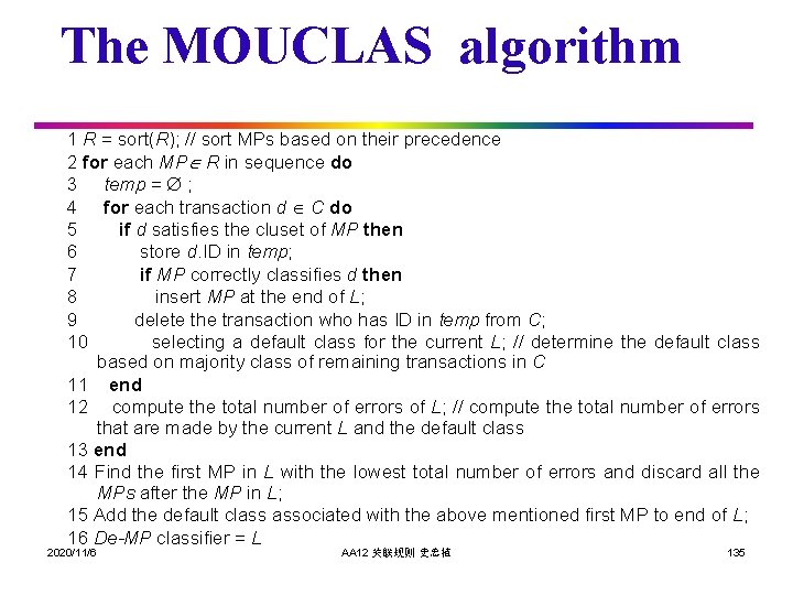
The MOUCLAS algorithm 1 R = sort(R); // sort MPs based on their precedence 2 for each MP R in sequence do 3 temp = ; 4 for each transaction d C do 5 if d satisfies the cluset of MP then 6 store d. ID in temp; 7 if MP correctly classifies d then 8 insert MP at the end of L; 9 delete the transaction who has ID in temp from C; 10 selecting a default class for the current L; // determine the default class based on majority class of remaining transactions in C 11 end 12 compute the total number of errors of L; // compute the total number of errors that are made by the current L and the default class 13 end 14 Find the first MP in L with the lowest total number of errors and discard all the MPs after the MP in L; 15 Add the default class associated with the above mentioned first MP to end of L; 16 De-MP classifier = L 2020/11/6 AA 12 关联规则 史忠植 135

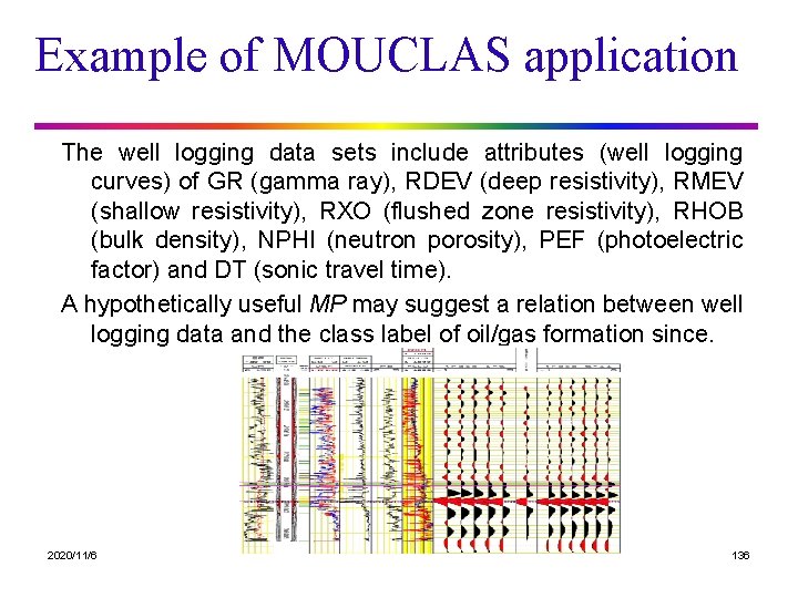
Example of MOUCLAS application The well logging data sets include attributes (well logging curves) of GR (gamma ray), RDEV (deep resistivity), RMEV (shallow resistivity), RXO (flushed zone resistivity), RHOB (bulk density), NPHI (neutron porosity), PEF (photoelectric factor) and DT (sonic travel time). A hypothetically useful MP may suggest a relation between well logging data and the class label of oil/gas formation since. 2020/11/6 AA 12 关联规则 史忠植 136

References l Jiawei Han and Micheline Kamber. Data Mining: Concepts and Techniques. Morgan Kaufmann Publishers l R. Agrawal, T. Imielinski, and A. Swami. Mining association rules between sets of items in large databases. SIGMOD'93, 207 -216, Washington, D. C. l J. Han, J. Pei, and Y. Yin: “Mining frequent patterns without candidate generation”. In Proc. ACM-SIGMOD’ 2000, pp. 112, Dallas, TX, May 2000. 2020/11/6 AA 12 关联规则 史忠植 138

References l S. Brin, R. Motwani, and C. Silverstein. Beyond market basket: Generalizing association rules to correlations. SIGMOD'97, 265276, Tucson, Arizona. l J. Han, L. V. S. Lakshmanan, and R. T. Ng, "Constraint-Based, Multidimensional Data Mining", COMPUTER (special issues on Data Mining), 32(8): 46 -50, 1999. l Craig A. Struble. Association Rule Mining. Slides, Marquette University l Yalei Hao. Markus Stumptner. Gerald Quirchmayr. Qing He. Data Mining by MOUCLAS Algorithm for Petroleum Reservoir Characterization from Well AA 12 Logging Data. AIAI 2004. 关联规则 史忠植 2020/11/6 139

www. intsci. ac. cn/shizz/ 2020/11/6 Questions? ! AA 12 关联规则 史忠植 140