L 5 Estimating Recombination Rates Review m M

L 5: Estimating Recombination Rates

Review § m. M: min. number of recombination events in any § § explanation of the haplotypes in M Last time, we covered 3 lower bounds on m. M The only exact algorithm that is known is super exponential. Not even an exponential time algorithm is known. Can we get efficient upper bounds that are tight. Idea: An Rs like method can be used to get an upper bound.

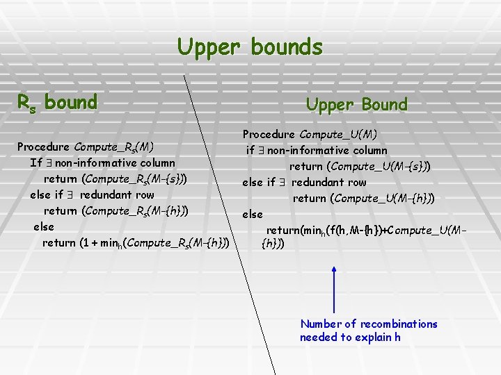
$Upper bounds Rs bound Procedure Compute_Rs(M) If non-informative column return (Compute_Rs(M-{s})) else if redundant$

Upper bounds Rs bound Procedure Compute_Rs(M) If non-informative column return (Compute_Rs(M-{s})) else if redundant row return (Compute_Rs(M-{h})) else return (1 + minh(Compute_Rs(M-{h})) Upper Bound Procedure Compute_U(M) if non-informative column return (Compute_U(M-{s})) else if redundant row return (Compute_U(M-{h})) else return(minh(f(h, M-{h})+Compute_U(M{h})) Number of recombinations needed to explain h

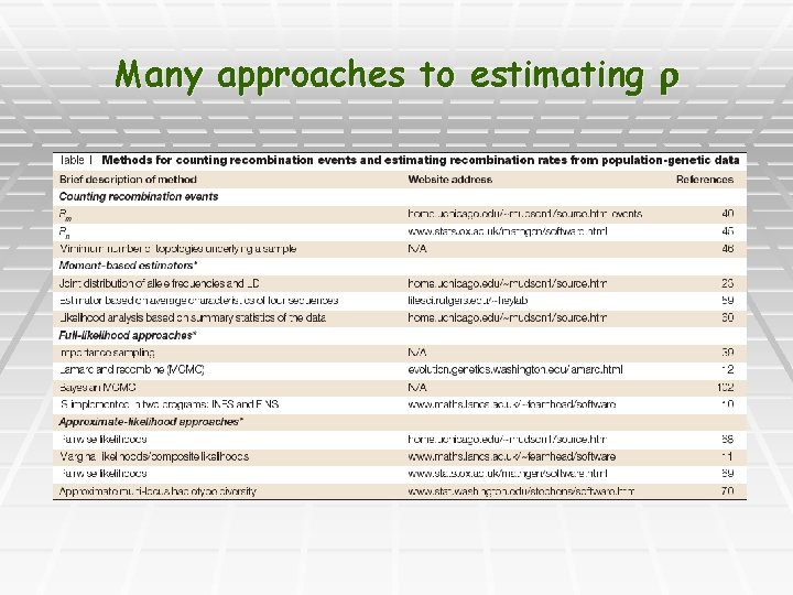
Many approaches to estimating

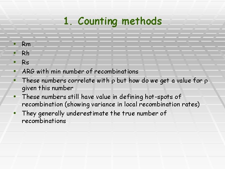
1. Counting methods Rm Rh Rs ARG with min number of recombinations These numbers correlate with but how do we get a value for given this number • These numbers still have value in defining hot-spots of recombination (showing variance in local recombination rates) • They generally underestimate the true number of recombinations • • •

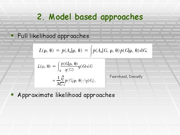
2. Model based approaches § Full likelihood approaches Fearnhead, Donnelly § Approximate likelihood approaches

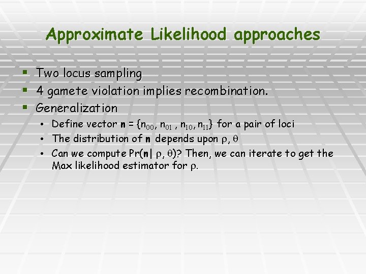
Approximate Likelihood approaches § Two locus sampling § 4 gamete violation implies recombination. § Generalization • • • Define vector n = {n 00, n 01 , n 10, n 11} for a pair of loci The distribution of n depends upon , Can we compute Pr(n| , )? Then, we can iterate to get the Max likelihood estimator for .

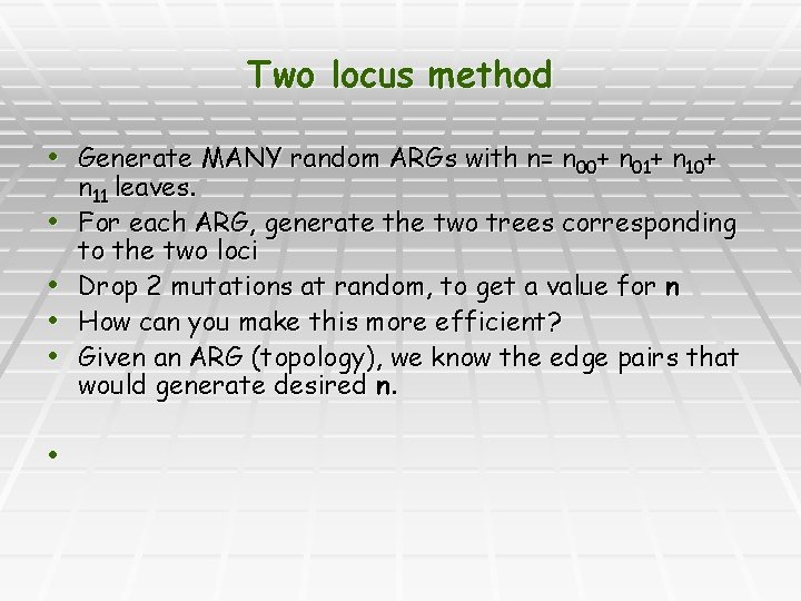
Two locus method • Generate MANY random ARGs with n= n 00+ n 01+ n 10+ • • • n 11 leaves. For each ARG, generate the two trees corresponding to the two loci Drop 2 mutations at random, to get a value for n How can you make this more efficient? Given an ARG (topology), we know the edge pairs that would generate desired n.

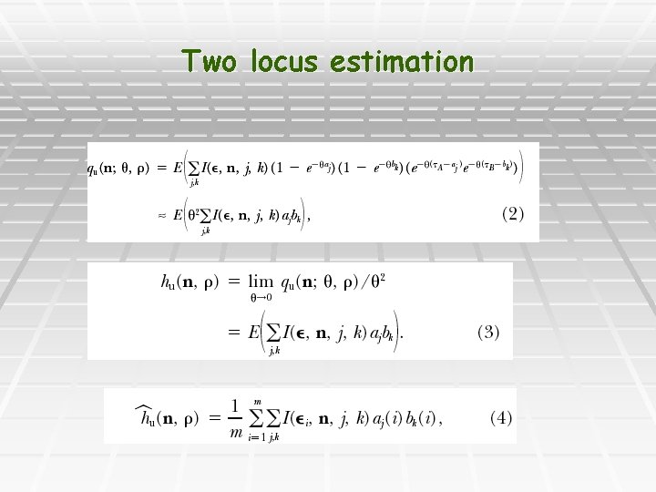
Two locus estimation

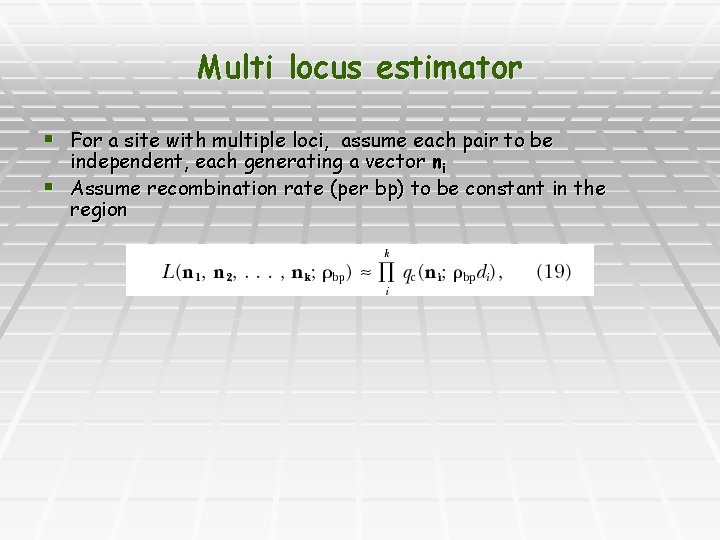
Multi locus estimator § For a site with multiple loci, assume each pair to be independent, each generating a vector ni § Assume recombination rate (per bp) to be constant in the region

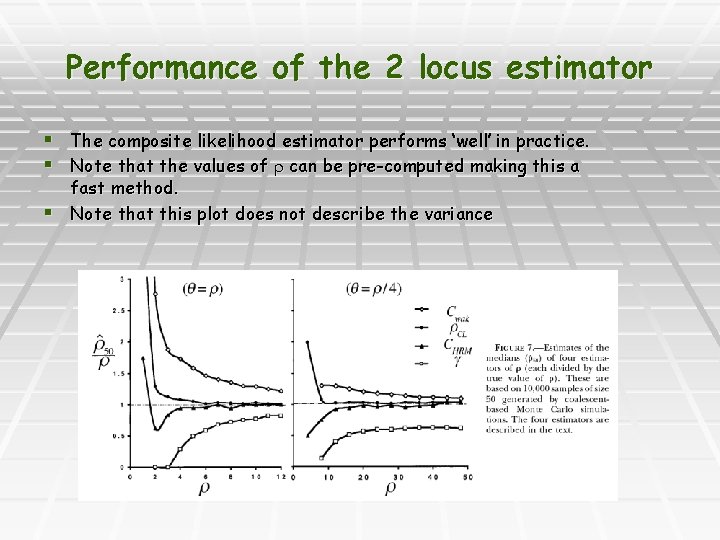
Performance of the 2 locus estimator § The composite likelihood estimator performs ‘well’ in practice. § Note that the values of can be pre-computed making this a fast method. § Note that this plot does not describe the variance

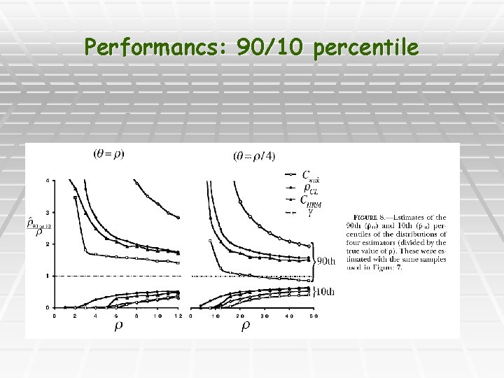
Performancs: 90/10 percentile

Research: 2 locus versus other statistics • Q 1: Can we use some of the counting based methods as summary statistic? • It is better than composite likelihood in that • It does not assume independence between loci. • There is a direct linear relationship (expected number of recombination events is log n) • Variation might be better. • Can we compute Pr(Rh| , ) efficiently? In a sense, it does not matter, because we can pre-compute the numbers. • Incorporate distance constraints in computing these summary statistics. It is reasonable to assume that the rate is constant per bp within a window.

Research Problem § Recombination hot-spots are NOT correlated between humans and Chimps. § 99% sequence identity § Virtually no overlap between hot-spots (generated using pop. Genetics). § What can cause this? § Method § Europeans/Africans share hot-spots § Concordance with sperm typing § Population sub-structure? Not (as shown by structure) § Genomic factors

Genomic factors § Recombination is elevated in GC rich regions § Epigenetic factors (such as acetylation, methylation) that affect chromatin structure might be key. § Yeast is a useful model for studying recombination § In yeast, recombination hotspots can be eliminated by insertion of transposable elements! § Can differential insertion of Alus explain the differences between chimps/humans?

Haplotype Phasing

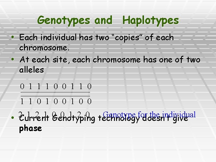
Genotypes and Haplotypes • Each individual has two “copies” of each chromosome. • At each site, each chromosome has one of two alleles 0 1 1 1 0 0 1 1 0 1 0 0 1 2 1 0 Genotyping 0 1 2 0 technology Genotype for the individual • 2 Current doesn’t give phase

§ Why is haplotype phasing important ?

Haplotype Phasing § Haplotype Phasing is the resolution of a genotype into the two haplotypes. § Haplotypes increase the power of an association between marker loci and phenotypic traits § Current approaches to Haplotyping § Via technological innovations (expensive) § Statistical Methods (ML, Phase, PL) § This lecture, we will consider a combinatorial approach to the phasing problem § Efficient, provable quality of solution § Not completely generalizable (as yet)

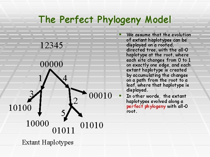
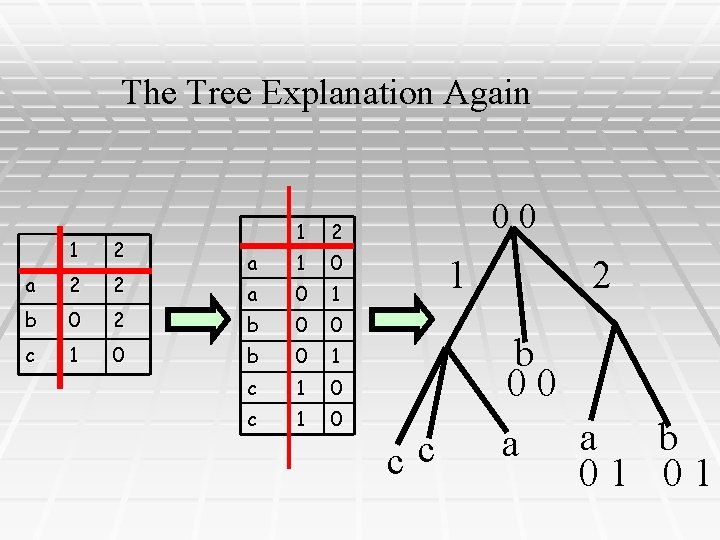
The Perfect Phylogeny Model § We assume that the evolution 12345 00000 1 4 3 10100 10000 2 00010 5 01011 Extant Haplotypes 01010 § of extant haplotypes can be displayed on a rooted, directed tree, with the all-0 haplotype at the root, where each site changes from 0 to 1 on exactly one edge, and each extant haplotype is created by accumulating the changes on a path from the root to a leaf, where that haplotype is displayed. In other words, the extant haplotypes evolved along a perfect phylogeny with all-0 root.

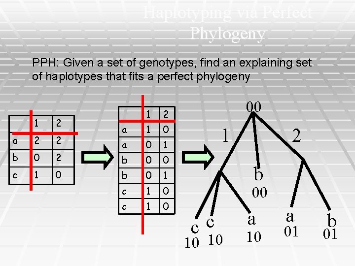
Haplotyping via Perfect Phylogeny PPH: Given a set of genotypes, find an explaining set of haplotypes that fits a perfect phylogeny 1 2 a 2 2 b 0 2 c 1 0 1 2 a 1 0 a 0 1 b 0 0 b 0 1 c 1 0 00 1 2 b 00 cc 10 10 a 01 b 01

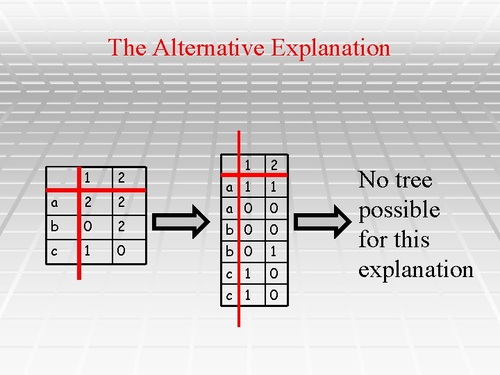
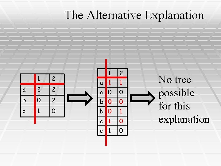
The Alternative Explanation 1 2 a 2 2 b 0 2 c 1 0 1 2 a 1 1 a 0 0 b 0 1 c 1 0 No tree possible for this explanation

The 4 Gamete Test for Perfect Phylogeny § Arrange the haplotypes in a matrix, two haplotypes for each individual. § Then (with no duplicate columns), the haplotypes fit a unique perfect phylogeny if and only if no two columns contain all four pairs (Buneman): 0, 0 and 0, 1 and 1, 0 and 1, 1 00 10 01 11

The Alternative Explanation 1 2 a 2 2 b 0 2 c 1 0 1 2 a 1 1 a 0 0 b 0 1 c 1 0 No tree possible for this explanation

The Tree Explanation Again 1 2 a 2 2 b 0 2 c 1 0 1 2 a 1 0 a 0 1 b 0 0 b 0 1 c 1 0 00 1 2 b 00 cc a a b 01 01

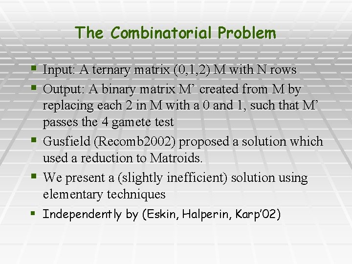
The Combinatorial Problem § Input: A ternary matrix (0, 1, 2) M with N rows § Output: A binary matrix M’ created from M by replacing each 2 in M with a 0 and 1, such that M’ passes the 4 gamete test § Gusfield (Recomb 2002) proposed a solution which used a reduction to Matroids. § We present a (slightly inefficient) solution using elementary techniques § Independently by (Eskin, Halperin, Karp’ 02)

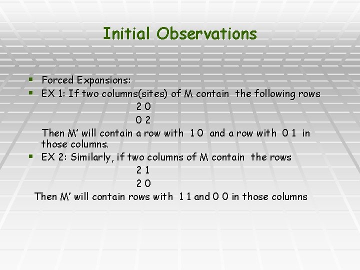
Initial Observations § Forced Expansions: § EX 1: If two columns(sites) of M contain the following rows 20 02 Then M’ will contain a row with 1 0 and a row with 0 1 in those columns. § EX 2: Similarly, if two columns of M contain the rows 21 20 Then M’ will contain rows with 1 1 and 0 0 in those columns

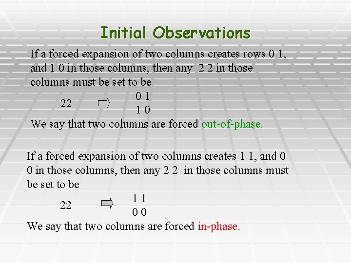
Initial Observations If a forced expansion of two columns creates rows 0 1, and 1 0 in those columns, then any 2 2 in those columns must be set to be 01 22 10 We say that two columns are forced out-of-phase. If a forced expansion of two columns creates 1 1, and 0 0 in those columns, then any 2 2 in those columns must be set to be 11 22 00 We say that two columns are forced in-phase.

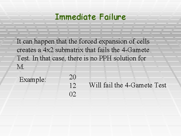
Immediate Failure It can happen that the forced expansion of cells creates a 4 x 2 submatrix that fails the 4 -Gamete Test. In that case, there is no PPH solution for M. 20 Example: Will fail the 4 -Gamete Test 12 02

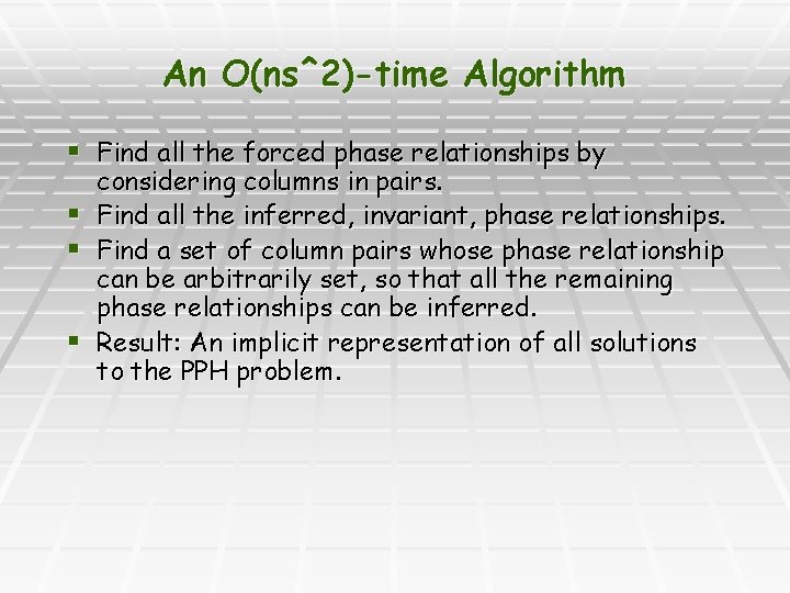
An O(ns^2)-time Algorithm § Find all the forced phase relationships by § § § considering columns in pairs. Find all the inferred, invariant, phase relationships. Find a set of column pairs whose phase relationship can be arbitrarily set, so that all the remaining phase relationships can be inferred. Result: An implicit representation of all solutions to the PPH problem.

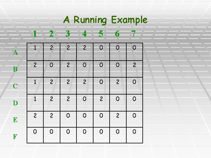
A B C D E F 1 A Running Example 2 3 4 5 6 7 1 2 2 2 0 0 0 2 1 2 2 2 0 1 2 2 0 0 0 0 0 0

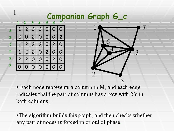
1 1 2 3 4 Companion Graph G_c 5 6 7 A 1 2 2 2 0 0 0 B 2 0 0 0 2 C 1 2 2 2 0 D 1 2 2 0 0 E 2 2 0 0 0 2 0 F 0 0 0 0 7 1 6 2 4 3 5 • Each node represents a column in M, and each edge indicates that the pair of columns has a row with 2’s in both columns. • The algorithm builds this graph, and then checks whether any pair of nodes is forced in or out of phase.

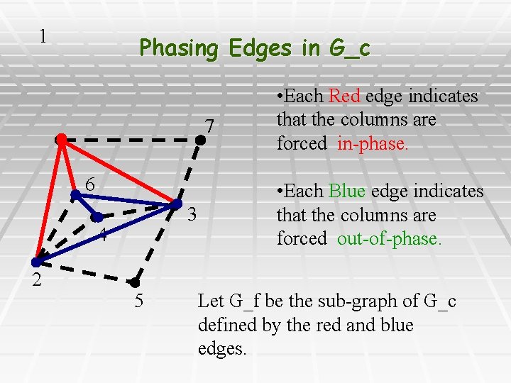
1 Phasing Edges in G_c 7 6 3 4 2 5 • Each Red edge indicates that the columns are forced in-phase. • Each Blue edge indicates that the columns are forced out-of-phase. Let G_f be the sub-graph of G_c defined by the red and blue edges.

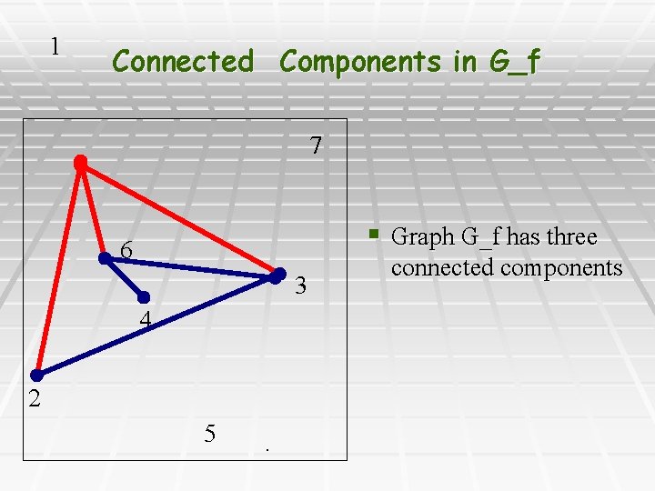
1 Connected Components in G_f 7 § Graph G_f has three 6 3 4 2 5 . connected components

Phase-parity Lemma § Lemma 1: There is a solution to the PPH problem for M if and only if there is a coloring of the black edges of G_c with the following property: For any triangle in G_c containing at least one black edge, the coloring makes either 0 or 2 of the edges blue (i. e. , out of phase) That’s nice, but how do we assign the colors?

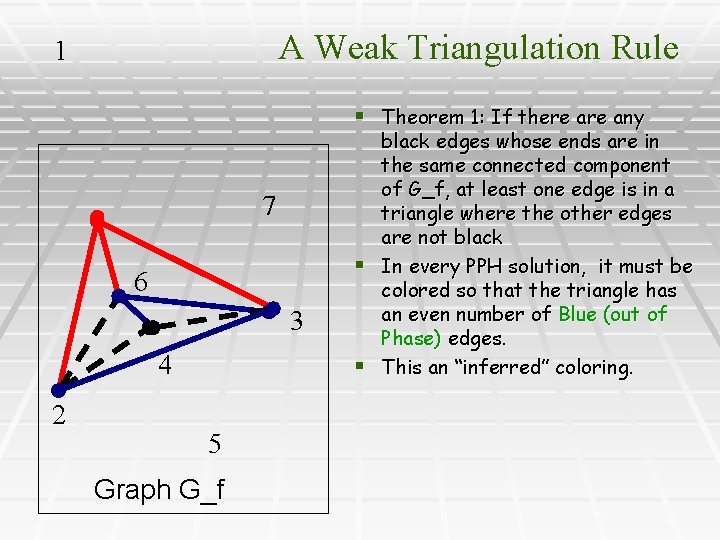
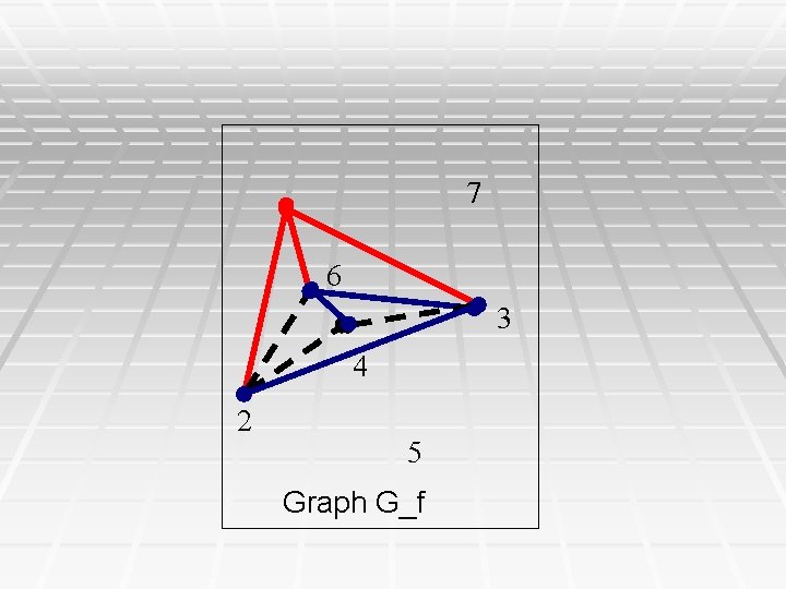
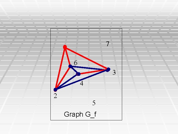
A Weak Triangulation Rule 1 § Theorem 1: If there any 7 6 3 4 2 5 Graph G_f black edges whose ends are in the same connected component of G_f, at least one edge is in a triangle where the other edges are not black § In every PPH solution, it must be colored so that the triangle has an even number of Blue (out of Phase) edges. § This an “inferred” coloring.

7 6 3 4 2 5 Graph G_f

Corollary § Inside any connected component of G_f, ALL the phase relationships on edges (columns of M) are uniquely determined, either as forced relationships based on pairwise column comparisons, or by triangle-based inferred colorings. § Hence, the phase relationships of all the columns in a connected component of G_f are INVARIANT over all the solutions to the PPH problem. § The black edges in G_f can be ordered so that the inferred colorings can be done in linear time. Modification of DFS.

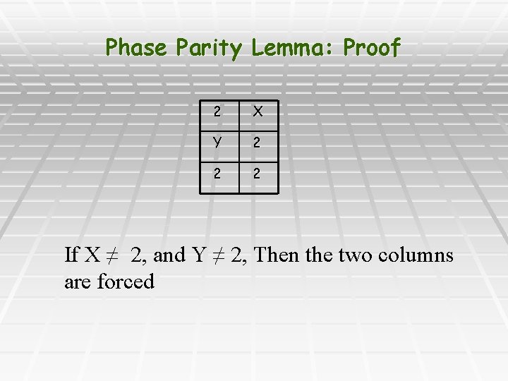
Phase Parity Lemma: Proof 2 X Y 2 2 2 If X ≠ 2, and Y ≠ 2, Then the two columns are forced

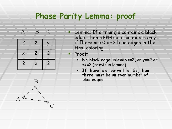
Phase Parity Lemma: proof A B C 2 2 y x 2 2 2 z 2 B A C § Lemma: If a triangle contains a black edge, then a PPH solution exists only if there are 0 or 2 blue edges in the final coloring. § Proof: § No black edge unless x==2, or y==2 or z==2 (previous lemma) § If there is a row with all 2 s, then there must be an even number of blue edges

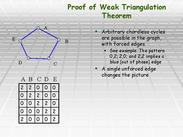
Proof of Weak Triangulation Theorem A § Arbitrary chordless cycles E B D C A B C D E 2 2 0 0 0 0 2 2 2 0 0 0 2 are possible in the graph, with forced edges. § See example. The pattern 0, 2; 2, 0; and 2, 2 implies a blue (out of phase) edge § A single unforced edge changes the picture

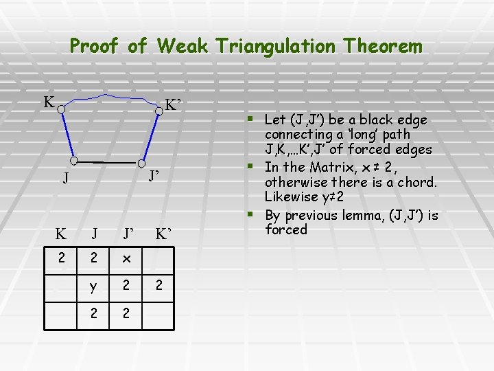
Proof of Weak Triangulation Theorem K K’ J’ J K J J’ 2 2 x y 2 2 2 K’ 2 § Let (J, J’) be a black edge connecting a ‘long’ path J, K, …K’, J’ of forced edges § In the Matrix, x ≠ 2, otherwise there is a chord. Likewise y≠ 2 § By previous lemma, (J, J’) is forced

Finishing the Solution Problem: A connected component C of G may contain several connected components of G_f, so any edge crossing two components of G_f will still be black. How should they be colored?

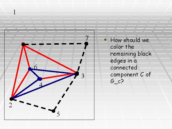
1 7 6 3 4 2 5 § How should we color the remaining black edges in a connected component C of G_c?

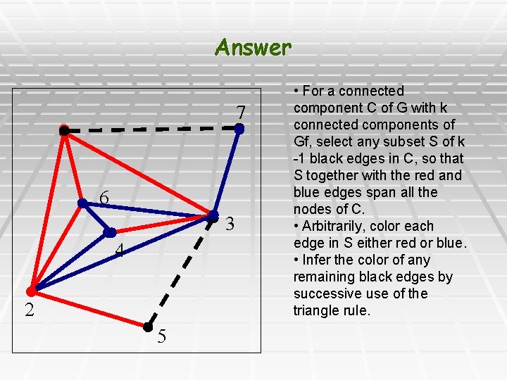
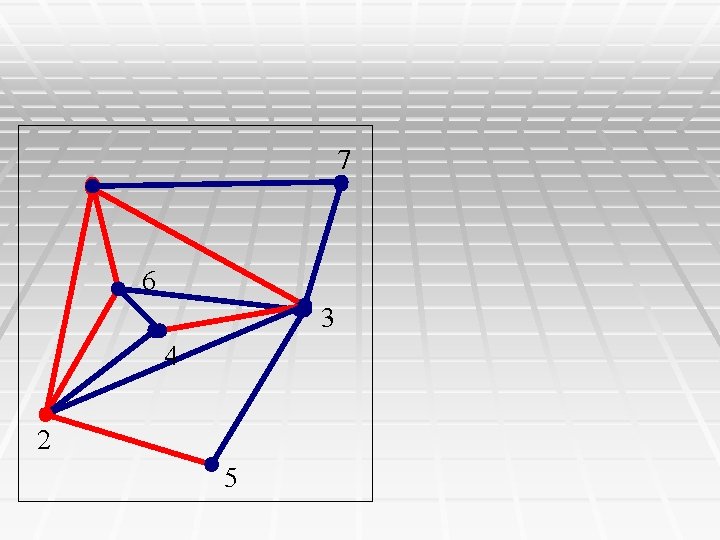
Answer 7 6 3 4 2 5 • For a connected component C of G with k connected components of Gf, select any subset S of k -1 black edges in C, so that S together with the red and blue edges span all the nodes of C. • Arbitrarily, color each edge in S either red or blue. • Infer the color of any remaining black edges by successive use of the triangle rule.

7 6 3 4 2 5

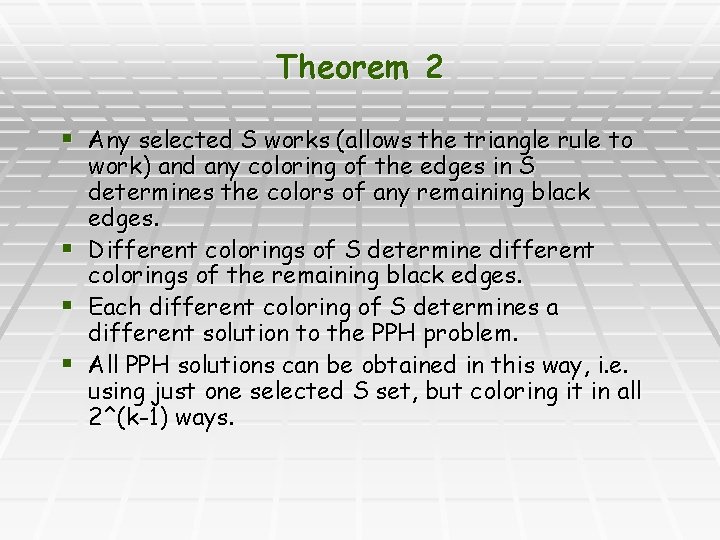
Theorem 2 § Any selected S works (allows the triangle rule to § § § work) and any coloring of the edges in S determines the colors of any remaining black edges. Different colorings of S determine different colorings of the remaining black edges. Each different coloring of S determines a different solution to the PPH problem. All PPH solutions can be obtained in this way, i. e. using just one selected S set, but coloring it in all 2^(k-1) ways.

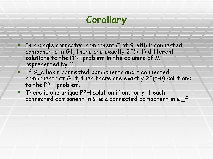
Corollary § In a single connected component C of G with k connected components in Gf, there are exactly 2^(k-1) different solutions to the PPH problem in the columns of M represented by C. § If G_c has r connected components and t connected components of G_f, then there are exactly 2^(t-r) solutions to the PPH problem. § There is one unique PPH solution if and only if each connected component in G is a connected component in G_f.

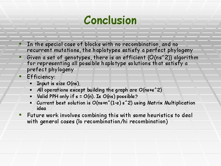
Conclusion § In the special case of blocks with no recombination, and no recurrent mutations, the haplotypes satisfy a perfect phylogeny § Given a set of genotypes, there is an efficient (O(ns^2)) algorithm for representing all possible haplotype solutions that satisfy a prefect phylogeny § Efficiency: § § Input is size O(ns), All operations except building the graph are O(ns+s^2) Valid PPH only if s = O(n). Is O(ns) possible? Current best solution is O(ns+n^(1 -e) s^2) using Matrix Multiplication idea § Future work involves combining this with some heuristics to deal with general cases (lo recombination/hi recombination)

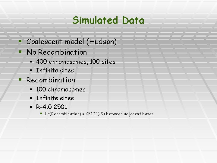
Simulated Data § Coalescent model (Hudson) § No Recombination § 400 chromosomes, 100 sites § Infinite sites § Recombination § § § 100 chromosomes Infinite sites R=4. 0 2501 § Pr(Recombination) = 4*10^(-9) between adjacent bases

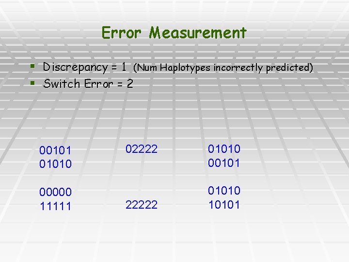
Error Measurement § Discrepancy = 1 (Num Haplotypes incorrectly predicted) § Switch Error = 2 001010 00000 11111 022222 01010 001010 10101

No Recombination

Choosing between solutions

Conclusion § Extremely low error rates (< 1% discrepancy) if no recombination § Randomly choosing between equivalent solutions is sufficient § Other measures (Parsimony, Likelihood, Entropy) do not improve the quality of solution

With Recombination