L 25 Working with Sound Files wavread sound

L 25. Working with Sound Files wavread sound wavwrite

Reading and Playing [y, rate, n. Bits] = wavread(‘no. Cry. wav’) sound(y, rate) How is audio information encoded? We will work with. wav files

Discrete vs Continuous Sound is continuous. Capture its essence by sampling. Digitized sound = 1 -dim array of numbers

Quality Issue: Sampling Rate If sampling not frequent enough, then the discretized sound will not capture the essence of the continuous sound… Too slow OK

Sampling Rate (Cont’d) Given human perception, about 20000 samples/second is pretty good. i. e. , 20000 Hertz i. e. , 20 k. HZ

Sampling Rate (Cont’d) 8, 000 Hz required for speech over the telephone 44, 100 Hz required for audio CD, MP 3 files 192, 400 Hz required for HD-DVD audio tracks

Quality Issue: Resolution Each sampled value is encoded as an eight-bit integer in the. wav file. Possible values: -128, -127, …, -1, 0, 1, …, 127 Loud: -120, 90, 122, etc Quiet: 3, 10, -5 8 -bits usually enough. Sometimes 16 -bits

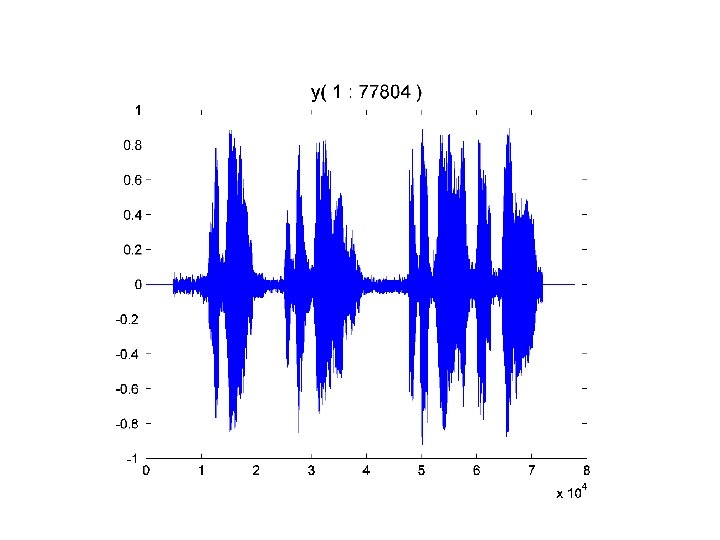
Back to wavread [y, rate, n. Bits] = wavread('no. Cry. wav'); n = length(y) n = 77804 rate = 11025 n. Bits = 8 no. Cry. wav encoded the sound with 77, 804 8 -bit numbers which were gathered over a span of about 77804/11025 secs

Let’s Look at the Sample Values 0. 07031250000000 -0. 13281250000000 -0. 67968750000000 -0. 5156250000 0. 2187500000 0. 4843750000 0. 71093750000000 0. 57031250000000 0. 14843750000000 0. 3906250000 0. 25000000 [y, rate, n. Bits] y(50000: 50010) values in between -1 and 1. = wavread(‘no. Cry. wav’)

Resolution with 8 Bits For each sample, wavread produces one of 256 possible floating point values: -1 256 possible values : -1 + k/128 +1

Let’s Plot the Digitized Sound [y, rate, n. Bits] = n = length(y) plot(y) wavread(‘no. Cry. wav’)

Summary Example: Name of the source file. [data, rate, n. Bits] = wavread(‘no. Cry. wav’) The vector of sampled sound values is assigned to this variable The sampling rate is assigned to this variable The resolution is assigned to this variable

Shortcuts [data, rate, n. Bits] = wavread(‘no. Cry. wav’) [data, rate] = wavread(‘no. Cry’) Usually don’t care about n. Bits Don’t need the. wav suffix

Playback via sound [data, rate]= wavread(‘no. Cry’) sound(data, rate) Usually want playback at a rate equal to the sampling rate.

To Compress or Not Compress The. wav format does not involve compression. The. mp 3 format does involve compression and it reduces storage by a factor of about 10.

Playlist Suppose we have a set of. wav files, e. g. , Casablanca. wav Austin. Powers. wav Gone. With. Wind. wav Back. To. School. wav and wish to play them in succession.

Three Problems 1. Making a Playlist. 2. Segmentation 3. Splicing

Problem 1: Making a Playlist Play. List = {'Casablanca', … 'Austin. Powers', … 'Gone. With. Wind', … 'Back. To. School'} for k=1: length(Play. List) [y, rate] = wavread(Play. List{k}); sound(y, rate) end Prob: Will start playing Austin Powers before Casablanca finishes.

Built-In Delays for k=1: length(Play. List) [y, rate] = wavread(Play. List{k}); sound(y, rate) L = length(y)/rate; pause(L+1) end Compute how long it’ll take and add one second.

Problem 2: Segmentation Are You Crying There is No crying There is No Crying In Baseball

Segmentation Are You Crying There is No crying There is No Crying In Baseball

Segmenting a. wav File Read in a. wav file. Display. Identify segments using mouseclicks. Store segments in a struct array.

Getting the Breakpoints [data, rate] = wavread(F); plot(data) [x, y] = ginput; x = floor(x); n. Segments = length(x)-1

Revisit ginput This solicits two mouseclicks: [x, y] = ginput(2) This solicits mouseclicks until the <return> key is pressed: [x, y] = ginput;

From Breakpoints to Subarray Extraction data: x: 2 7 19 29 Breakpoint array via ginput

From Breakpoints to Subarray Extraction data: 7: 18 2: 6 x: 2 7 19 For kth segment: First = x(k); 19: 28 29 Last = x(k+1)-1

Setting up the Struct Array for k=1: n. Segments First = x(k); Last = x(k+1)-1; z = data(First: Last); C(k) = struct('rate', rate, … 'z', z); end

Playing the Segments function Play. Segments(C) for k=1: length(C) the. Data = C(k). z; the. Rate = C(k). rate; sound(the. Data, the. Rate) pause(length(the. Data)/the. Rate +1) end That’s how long it takes the Kth segment to play.

Making a. wav File Suppose C is a struct array consisting of N sound segments all sampled at the same Rate. Make a single. wav file that plays the segments in reverse order.

Reversing the Segments function Reverse(C, F) n = length(C); y = []; for k = 1: n y = [ C(k). z ; y]; end wavwrite(y, C(1). rate, 8, [F '. wav']);

wavwrite(data, rate, n. Bits, fname) Target file, e. g. , ‘F. wav’