L 16 Microarray analysis Dimension reduction Unsupervised clustering

L 16: Micro-array analysis Dimension reduction Unsupervised clustering

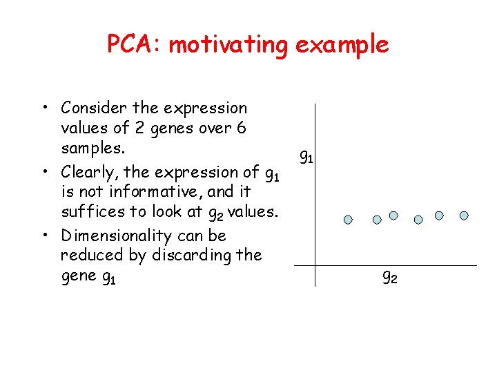
PCA: motivating example • Consider the expression values of 2 genes over 6 samples. • Clearly, the expression of g 1 is not informative, and it suffices to look at g 2 values. • Dimensionality can be reduced by discarding the gene g 1 g 2

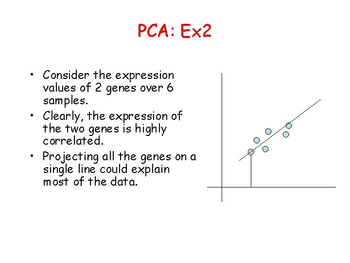
PCA: Ex 2 • Consider the expression values of 2 genes over 6 samples. • Clearly, the expression of the two genes is highly correlated. • Projecting all the genes on a single line could explain most of the data.

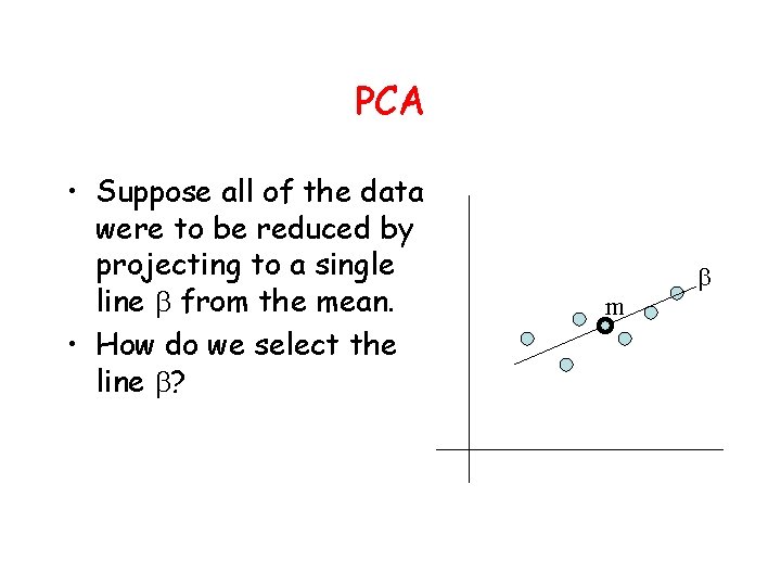
PCA • Suppose all of the data were to be reduced by projecting to a single line from the mean. • How do we select the line ? m

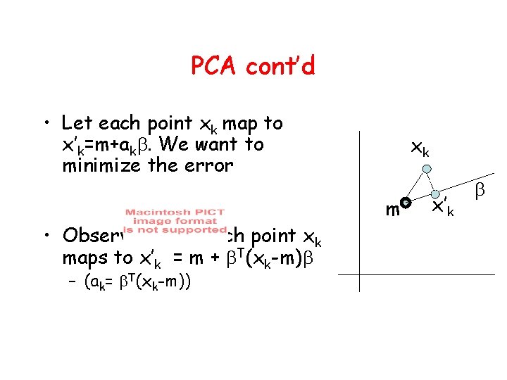
PCA cont’d • Let each point xk map to x’k=m+ak. We want to minimize the error • Observation 1: Each point xk maps to x’k = m + T(xk-m) – (ak= T(xk-m)) xk m x’k

Proof of Observation 1 Differentiating w. r. t ak

Minimizing PCA Error • To minimize error, we must maximize TS • By definition, = TS implies that is an eigenvalue, and the corresponding eigenvector. • Therefore, we must choose the eigenvector corresponding to the largest eigenvalue.

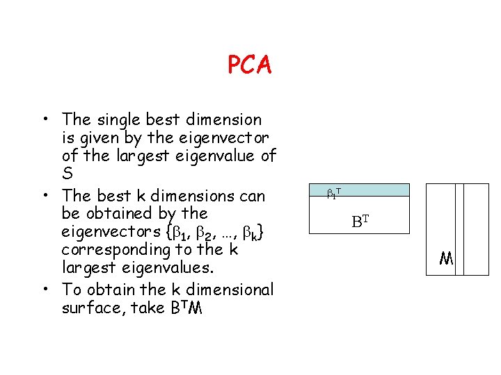
PCA • The single best dimension is given by the eigenvector of the largest eigenvalue of S • The best k dimensions can be obtained by the eigenvectors { 1, 2, …, k} corresponding to the k largest eigenvalues. • To obtain the k dimensional surface, take BTM 1 T BT M

Clustering • Suppose we are not given any classes. • Instead, we are asked to partition the samples into clusters that make sense. • Alternatively, partition genes into clusters. • Clustering is part of unsupervised learning

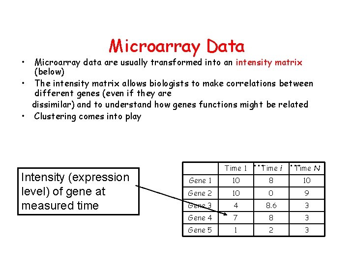
• Microarray Data Microarray data are usually transformed into an intensity matrix (below) • The intensity matrix allows biologists to make correlations between different genes (even if they are dissimilar) and to understand how genes functions might be related • Clustering comes into play Intensity (expression level) of gene at measured time Time 1 …Time i … Time N Gene 1 10 8 10 Gene 2 10 0 9 Gene 3 4 8. 6 3 Gene 4 7 8 3 Gene 5 1 2 3

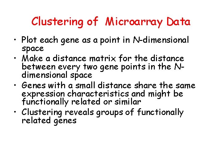
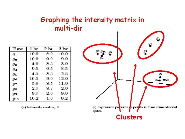
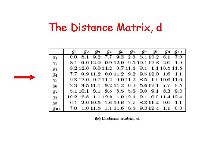
Clustering of Microarray Data • Plot each gene as a point in N-dimensional space • Make a distance matrix for the distance between every two gene points in the Ndimensional space • Genes with a small distance share the same expression characteristics and might be functionally related or similar • Clustering reveals groups of functionally related genes

Graphing the intensity matrix in multi-dimensional space Clusters

The Distance Matrix, d

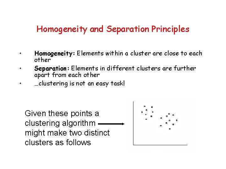
Homogeneity and Separation Principles • • • Homogeneity: Elements within a cluster are close to each other Separation: Elements in different clusters are further apart from each other …clustering is not an easy task! Given these points a clustering algorithm might make two distinct clusters as follows

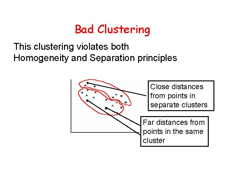
Bad Clustering This clustering violates both Homogeneity and Separation principles Close distances from points in separate clusters Far distances from points in the same cluster

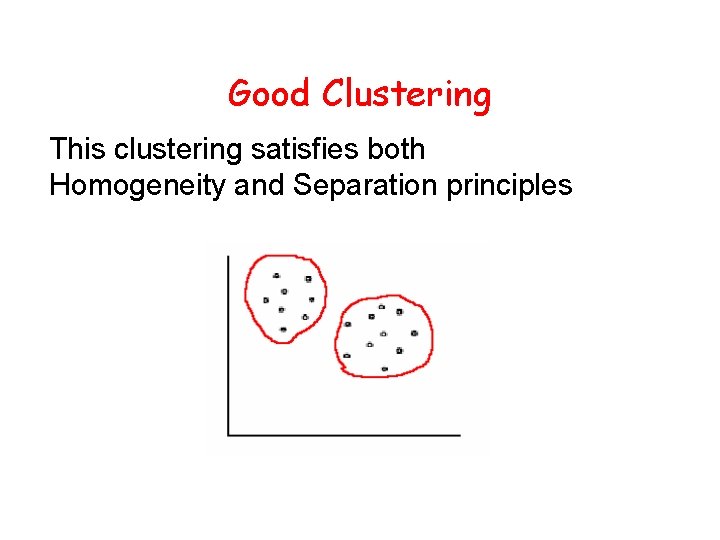
Good Clustering This clustering satisfies both Homogeneity and Separation principles

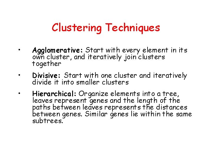
Clustering Techniques • Agglomerative: Start with every element in its own cluster, and iteratively join clusters together • Divisive: Start with one cluster and iteratively divide it into smaller clusters • Hierarchical: Organize elements into a tree, leaves represent genes and the length of the paths between leaves represents the distances between genes. Similar genes lie within the same subtrees.

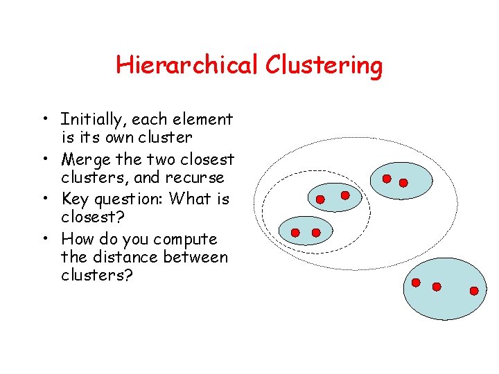
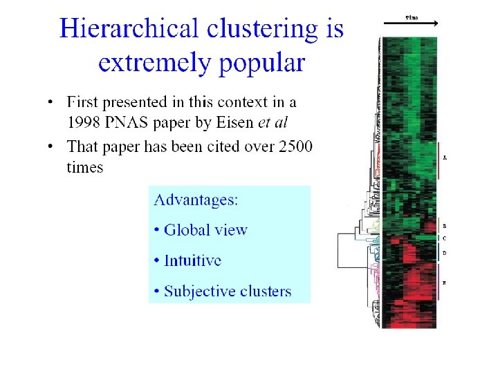
Hierarchical Clustering • Initially, each element is its own cluster • Merge the two closest clusters, and recurse • Key question: What is closest? • How do you compute the distance between clusters?

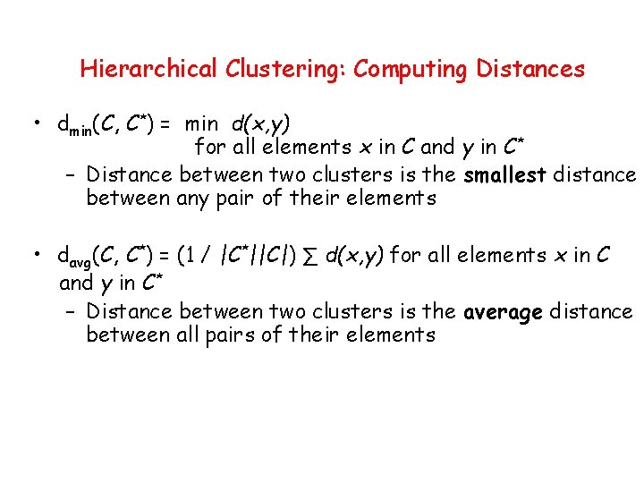
Hierarchical Clustering: Computing Distances • dmin(C, C*) = min d(x, y) for all elements x in C and y in C* – Distance between two clusters is the smallest distance between any pair of their elements • davg(C, C*) = (1 / |C*||C|) ∑ d(x, y) for all elements x in C and y in C* – Distance between two clusters is the average distance between all pairs of their elements

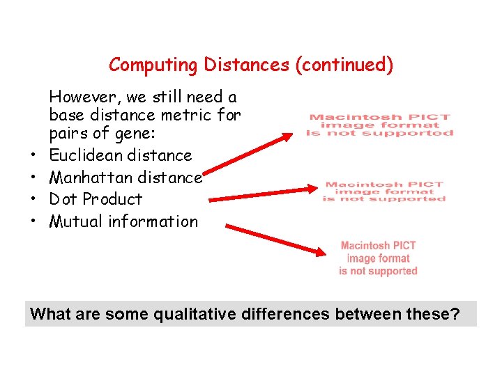
Computing Distances (continued) • • However, we still need a base distance metric for pairs of gene: Euclidean distance Manhattan distance Dot Product Mutual information What are some qualitative differences between these?

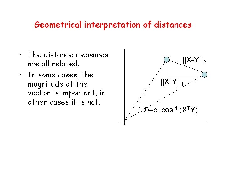
Geometrical interpretation of distances • The distance measures are all related. • In some cases, the magnitude of the vector is important, in other cases it is not. ||X-Y||2 ||X-Y||1 =c. cos-1 (XTY)

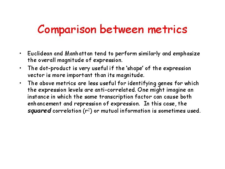
Comparison between metrics • • • Euclidean and Manhattan tend to perform similarly and emphasize the overall magnitude of expression. The dot-product is very useful if the ‘shape’ of the expression vector is more important than its magnitude. The above metrics are less useful for identifying genes for which the expression levels are anti-correlated. One might imagine an instance in which the same transcription factor can cause both enhancement and repression of expression. In this case, the squared correlation (r 2) or mutual information is sometimes used.

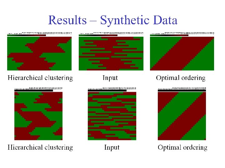
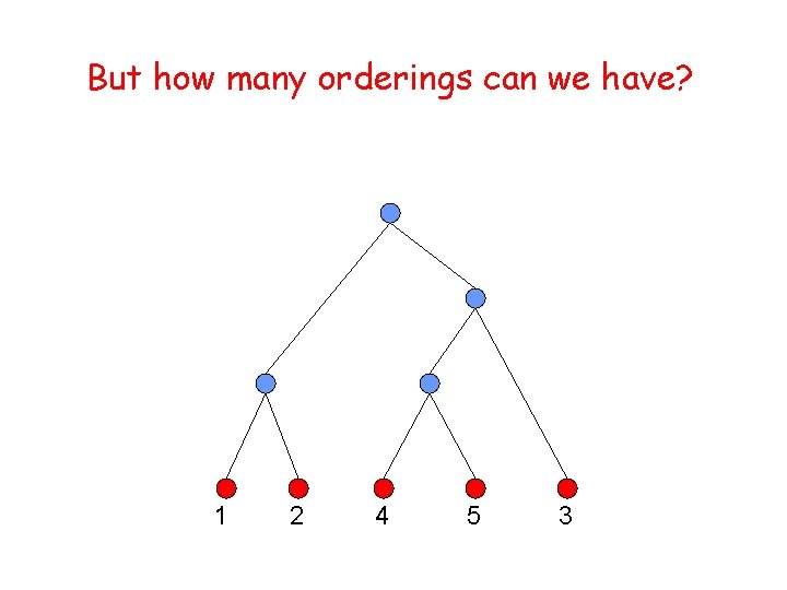
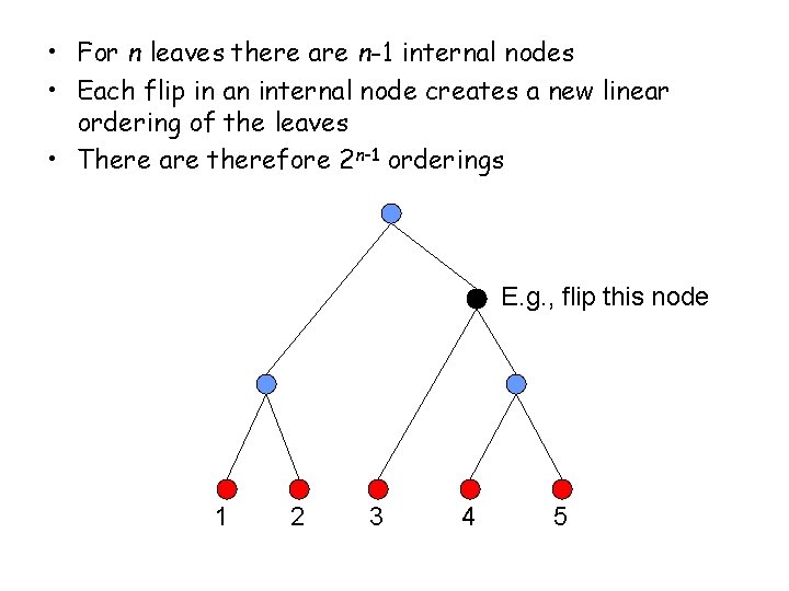
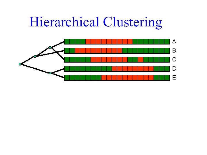
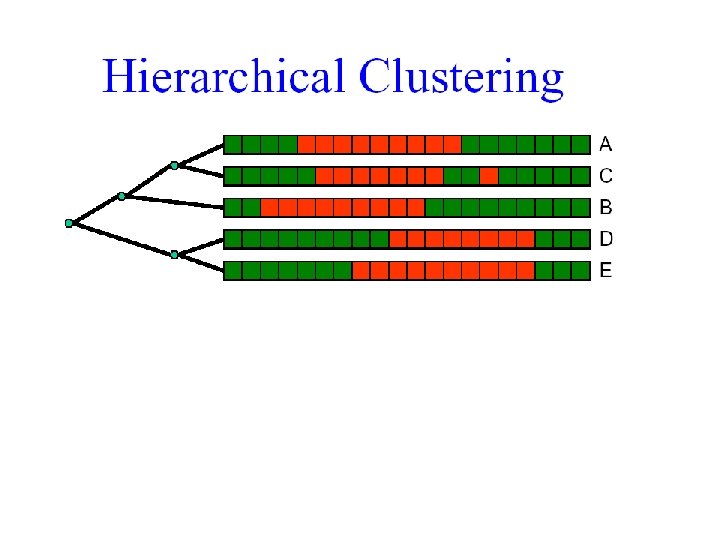
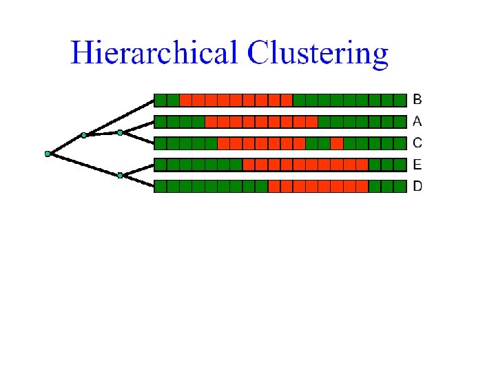
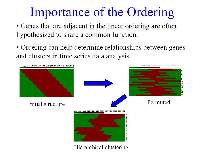
But how many orderings can we have? 1 2 4 5 3

• For n leaves there are n-1 internal nodes • Each flip in an internal node creates a new linear ordering of the leaves • There are therefore 2 n-1 orderings E. g. , flip this node 1 2 3 4 5

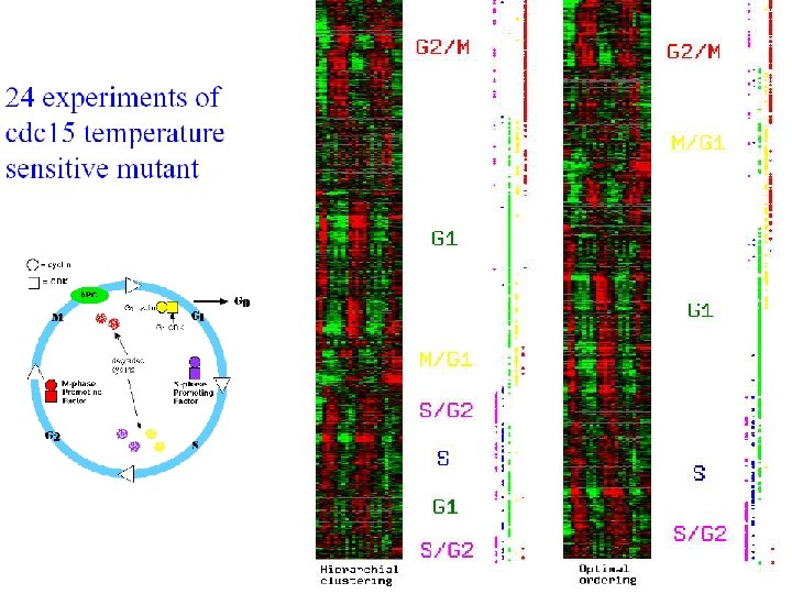
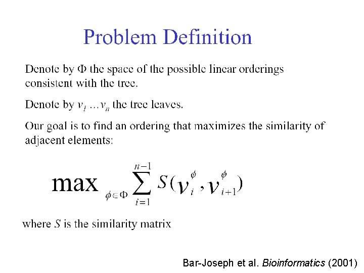
Bar-Joseph et al. Bioinformatics (2001)

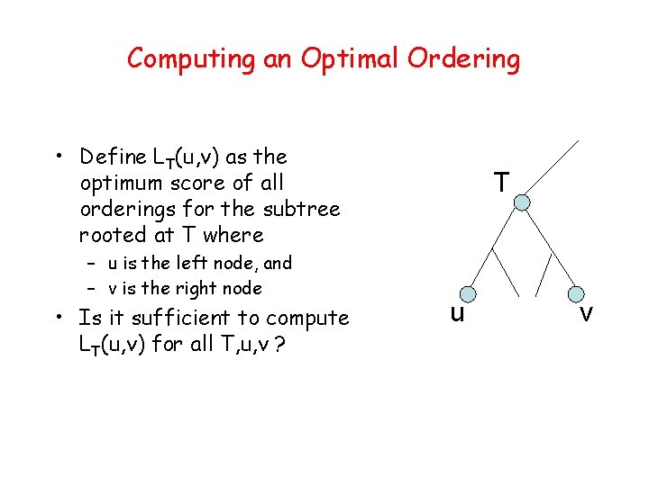
Computing an Optimal Ordering • Define LT(u, v) as the optimum score of all orderings for the subtree rooted at T where – u is the left node, and – v is the right node • Is it sufficient to compute LT(u, v) for all T, u, v ? T u v

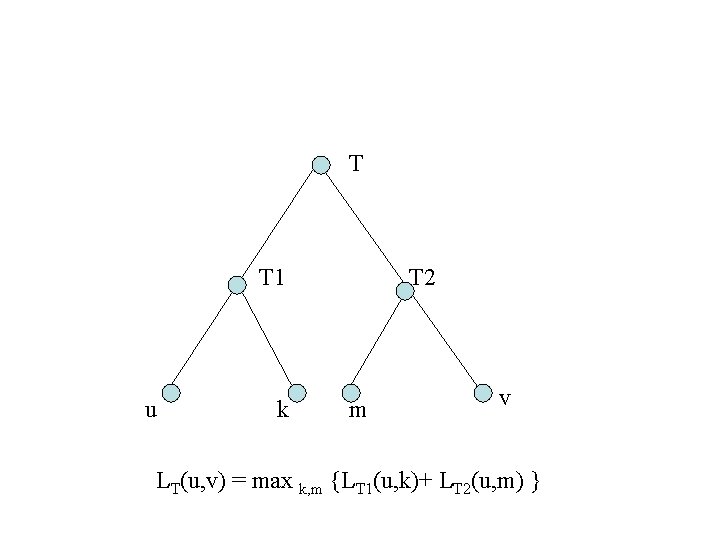
T T 1 u k T 2 m v LT(u, v) = max k, m {LT 1(u, k)+ LT 2(u, m) }

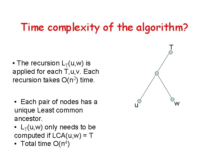
Time complexity of the algorithm? T • The recursion LT(u, w) is applied for each T, u, v. Each recursion takes O(n 2) time. • Each pair of nodes has a unique Least common ancestor. • LT(u, w) only needs to be computed if LCA(u, w) = T • Total time O(n 4) u w

Speed Improvements • For all m in LT 1(u, R) – If LT 1(u, m)+LT 2(k 0, w)+ C(T 1, T 2) <= Curr. Max • Exit loop – For all k in LT 1(w, L) • If LT 1(u, m)+LT 2(k, w)+C(T 1, T 2) <= Curr. Max – Exit loop • Else recompute Curr. Max. • In practice, this leads to great speed improvements • 1500 genes, 7 hrs. changes to 7 min.