L 132 Microsoft Excel Formulas Formatting and Creating

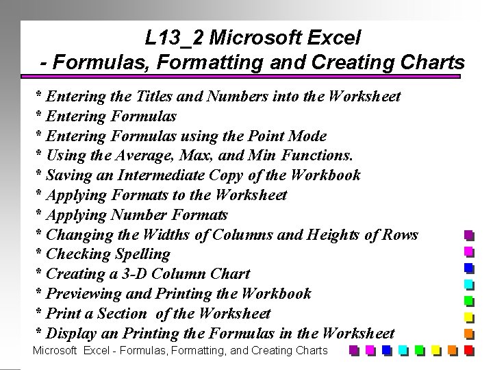
L 13_2 Microsoft Excel - Formulas, Formatting and Creating Charts * Entering the Titles and Numbers into the Worksheet * Entering Formulas using the Point Mode * Using the Average, Max, and Min Functions. * Saving an Intermediate Copy of the Workbook * Applying Formats to the Worksheet * Applying Number Formats * Changing the Widths of Columns and Heights of Rows * Checking Spelling * Creating a 3 -D Column Chart * Previewing and Printing the Workbook * Print a Section of the Worksheet * Display an Printing the Formulas in the Worksheet Microsoft Excel - Formulas, Formatting, and Creating Charts

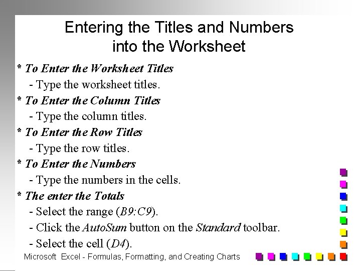
Entering the Titles and Numbers into the Worksheet * To Enter the Worksheet Titles - Type the worksheet titles. * To Enter the Column Titles - Type the column titles. * To Enter the Row Titles - Type the row titles. * To Enter the Numbers - Type the numbers in the cells. * The enter the Totals - Select the range (B 9: C 9). - Click the Auto. Sum button on the Standard toolbar. - Select the cell (D 4). Microsoft Excel - Formulas, Formatting, and Creating Charts

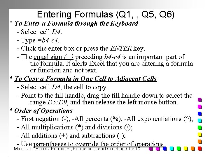
Entering Formulas (Q 1, , Q 5, Q 6) * To Enter a Formula through the Keyboard - Select cell D 4. - Type =b 4 -c 4. - Click the enter box or press the ENTER key. - The equal sign (=) preceding b 4 -c 4 is an important part of the formula. It alerts Excel that you are entering a formula or function and not text. * To Copy a Formula in One Cell to Adjacent Cells - Select cell D 4, the sell to copy. - Point to the fill handle, drag the fill handle down to select the range D 5: D 9, and then release the left mouse button. * Order of Operations - First negation (-); -All percents (%); -All exponentiations (^); - All multiplications (*) and divisions (/); - All additions (+) and subtractions (-); - Use parentheses to override the order of operations. Microsoft Excel - Formulas, Formatting, and Creating Charts

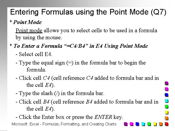
Entering Formulas using the Point Mode (Q 7) * Point Mode Point mode allows you to select cells to be used in a formula by using the mouse. * To Enter a Formula “=C 4/B 4” in E 4 Using Point Mode - Select cell E 4. - Type the equal sign (=) in the formula bar to begin the formula. - Click cell C 4 (cell reference C 4 added to formula bar and in the cell E 4). - Type the slash (/) in the formula bar. - Click cell B 4 (cell reference B 4 added to formula bar and in the cell E 4). - Click the Enter box or press the ENTER key. Microsoft Excel - Formulas, Formatting, and Creating Charts

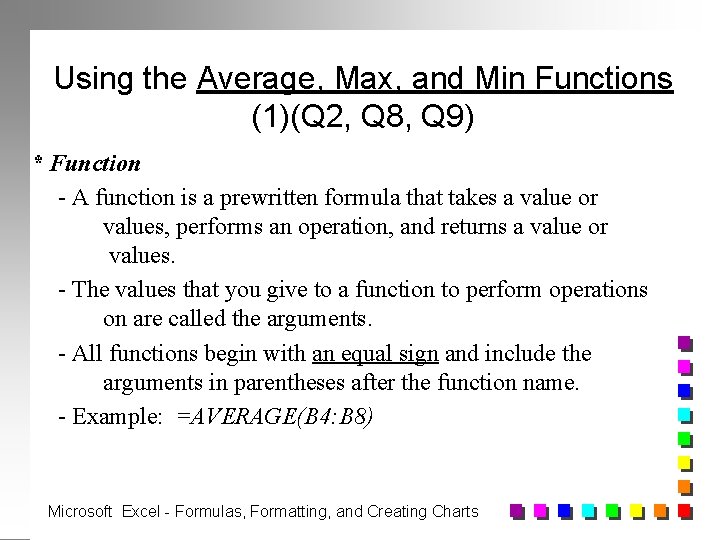
Using the Average, Max, and Min Functions (1)(Q 2, Q 8, Q 9) * Function - A function is a prewritten formula that takes a value or values, performs an operation, and returns a value or values. - The values that you give to a function to perform operations on are called the arguments. - All functions begin with an equal sign and include the arguments in parentheses after the function name. - Example: =AVERAGE(B 4: B 8) Microsoft Excel - Formulas, Formatting, and Creating Charts

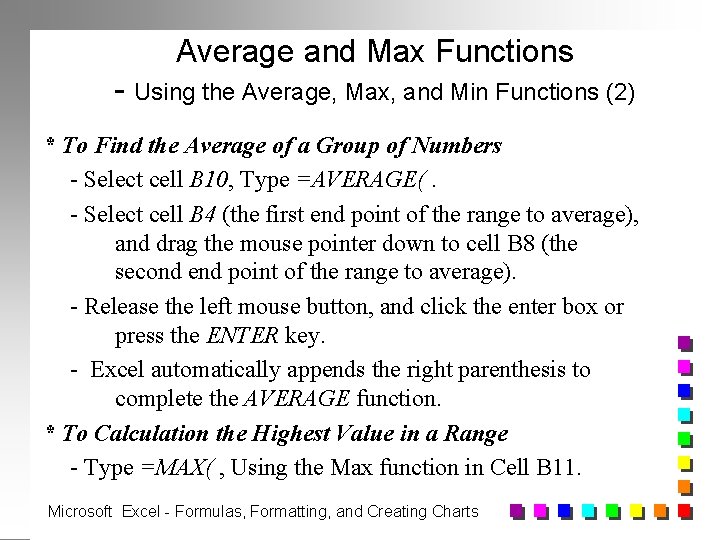
Average and Max Functions - Using the Average, Max, and Min Functions (2) * To Find the Average of a Group of Numbers - Select cell B 10, Type =AVERAGE(. - Select cell B 4 (the first end point of the range to average), and drag the mouse pointer down to cell B 8 (the second end point of the range to average). - Release the left mouse button, and click the enter box or press the ENTER key. - Excel automatically appends the right parenthesis to complete the AVERAGE function. * To Calculation the Highest Value in a Range - Type =MAX( , Using the Max function in Cell B 11. Microsoft Excel - Formulas, Formatting, and Creating Charts

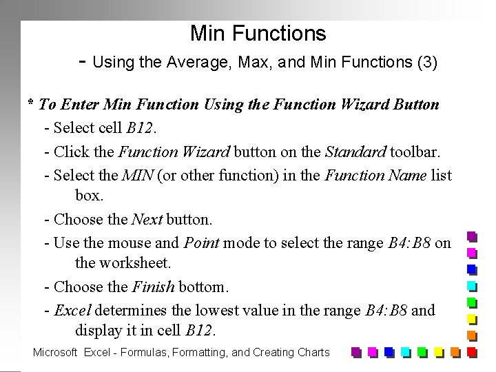
Min Functions - Using the Average, Max, and Min Functions (3) * To Enter Min Function Using the Function Wizard Button - Select cell B 12. - Click the Function Wizard button on the Standard toolbar. - Select the MIN (or other function) in the Function Name list box. - Choose the Next button. - Use the mouse and Point mode to select the range B 4: B 8 on the worksheet. - Choose the Finish bottom. - Excel determines the lowest value in the range B 4: B 8 and display it in cell B 12. Microsoft Excel - Formulas, Formatting, and Creating Charts

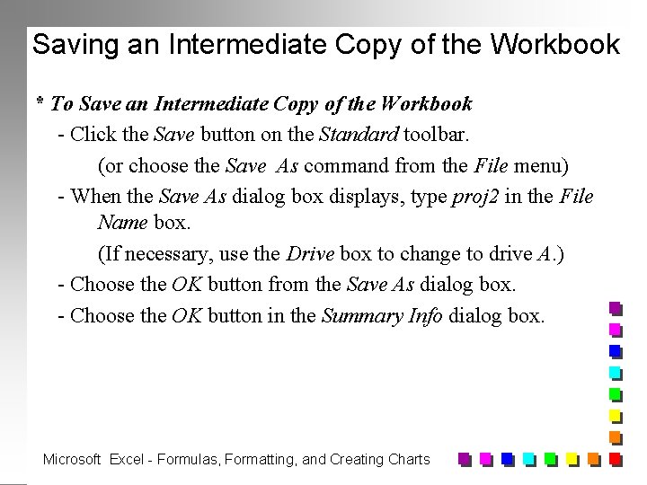
Saving an Intermediate Copy of the Workbook * To Save an Intermediate Copy of the Workbook - Click the Save button on the Standard toolbar. (or choose the Save As command from the File menu) - When the Save As dialog box displays, type proj 2 in the File Name box. (If necessary, use the Drive box to change to drive A. ) - Choose the OK button from the Save As dialog box. - Choose the OK button in the Summary Info dialog box. Microsoft Excel - Formulas, Formatting, and Creating Charts

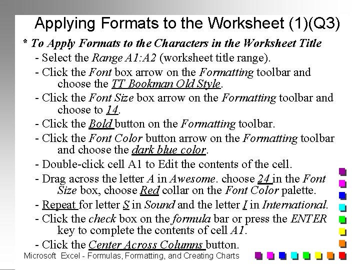
Applying Formats to the Worksheet (1)(Q 3) * To Apply Formats to the Characters in the Worksheet Title - Select the Range A 1: A 2 (worksheet title range). - Click the Font box arrow on the Formatting toolbar and choose the TT Bookman Old Style. - Click the Font Size box arrow on the Formatting toolbar and choose to 14. - Click the Bold button on the Formatting toolbar. - Click the Font Color button arrow on the Formatting toolbar and choose the dark blue color. - Double-click cell A 1 to Edit the contents of the cell. - Drag across the letter A in Awesome. choose 24 in the Font Size box, choose Red collar on the Font Color palette. - Repeat for letter S in Sound and the letter I in International. - Click the check box on the formula bar or press the ENTER key to complete the contents of cell A 1. - Click the Center Across Columns button. Microsoft Excel - Formulas, Formatting, and Creating Charts

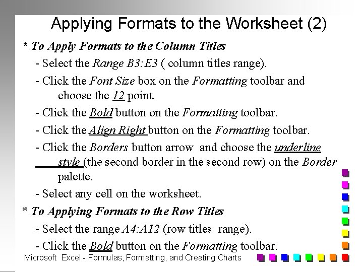
Applying Formats to the Worksheet (2) * To Apply Formats to the Column Titles - Select the Range B 3: E 3 ( column titles range). - Click the Font Size box on the Formatting toolbar and choose the 12 point. - Click the Bold button on the Formatting toolbar. - Click the Align Right button on the Formatting toolbar. - Click the Borders button arrow and choose the underline style (the second border in the second row) on the Border palette. - Select any cell on the worksheet. * To Applying Formats to the Row Titles - Select the range A 4: A 12 (row titles range). - Click the Bold button on the Formatting toolbar. Microsoft Excel - Formulas, Formatting, and Creating Charts

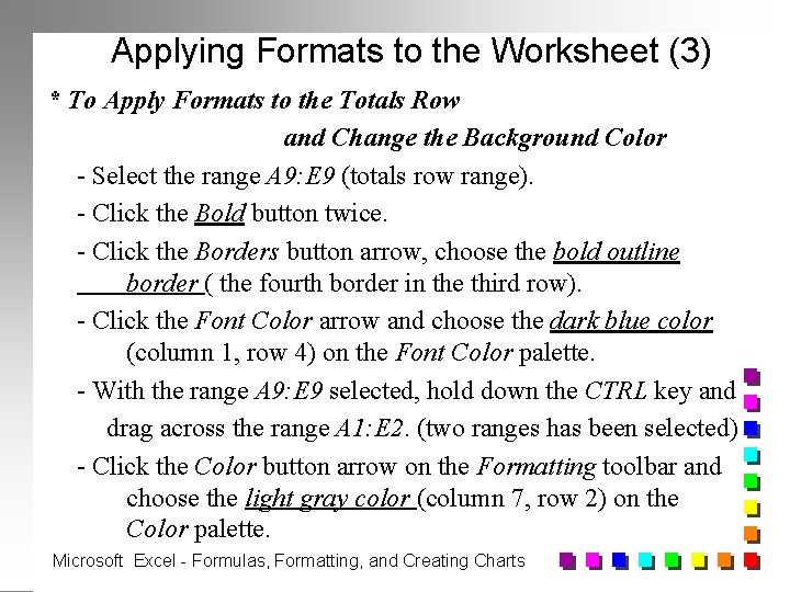
Applying Formats to the Worksheet (3) * To Apply Formats to the Totals Row and Change the Background Color - Select the range A 9: E 9 (totals row range). - Click the Bold button twice. - Click the Borders button arrow, choose the bold outline border ( the fourth border in the third row). - Click the Font Color arrow and choose the dark blue color (column 1, row 4) on the Font Color palette. - With the range A 9: E 9 selected, hold down the CTRL key and drag across the range A 1: E 2. (two ranges has been selected) - Click the Color button arrow on the Formatting toolbar and choose the light gray color (column 7, row 2) on the Color palette. Microsoft Excel - Formulas, Formatting, and Creating Charts

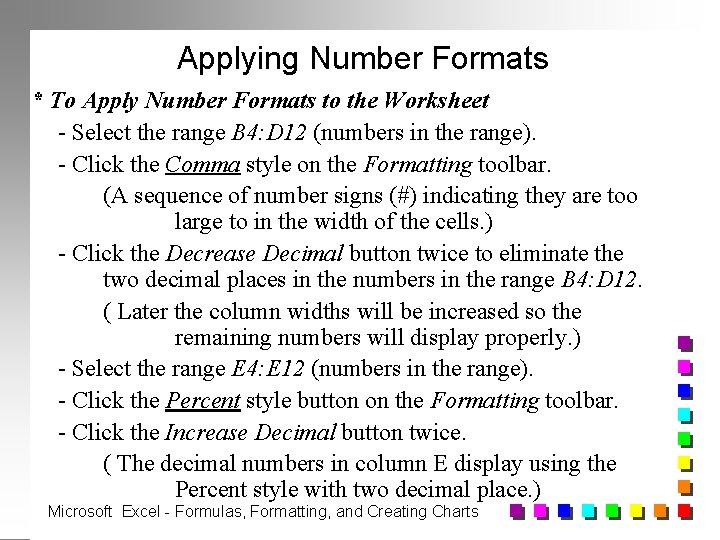
Applying Number Formats * To Apply Number Formats to the Worksheet - Select the range B 4: D 12 (numbers in the range). - Click the Comma style on the Formatting toolbar. (A sequence of number signs (#) indicating they are too large to in the width of the cells. ) - Click the Decrease Decimal button twice to eliminate the two decimal places in the numbers in the range B 4: D 12. ( Later the column widths will be increased so the remaining numbers will display properly. ) - Select the range E 4: E 12 (numbers in the range). - Click the Percent style button on the Formatting toolbar. - Click the Increase Decimal button twice. ( The decimal numbers in column E display using the Percent style with two decimal place. ) Microsoft Excel - Formulas, Formatting, and Creating Charts

Changing the Widths of Columns and Heights of Rows (1) * Default Width and Height - Default width is 8. 43 character. A character is defined as TT Arial 10 point. - Default height is 12. 75 points. A single point is about 1/72 of one inch. * To Change the Width of a Column to Best Fit - Position the mouse pointer on the border line between the column A and column B headings above row 1. ( the Mouse pointer becomes a split double arrow. ) - Double-click the left mouse button. (The width of column A increases just enough so the widest entry in column A, Latin American, fits in cell A 7. ) Microsoft Excel - Formulas, Formatting, and Creating Charts

Changing the Widths of Columns and Heights of Rows (2)(Q 10) * To Change the Width of a Column - Position the mouse pointer on the border line between the column B and column C headings above row 1. - Drag the mouse pointer to the right until the number 13. 71 displays in the reference area in the formula bar. - Release the left mouse button. Microsoft Excel - Formulas, Formatting, and Creating Charts

Changing the Widths of Columns and Heights of Rows (3) * To Change the Width of More than One Columns - Drag the mouse pointer from column heading C through column heading D and release the left mouse button to select both columns. - Move the mouse pointer to the right border of column heading D. - When the mouse pointer changes to a split double arrow, drag to the right until a width of 11. 00 displays in the reference area in the formula bar. - Release the left mouse button. Microsoft Excel - Formulas, Formatting, and Creating Charts

Changing the Widths of Columns and Heights of Rows (4) * To Change the Width of a Column Using Shortcut Menu - Click column heading E to select the column. - Click the right mouse button to display the shortcut menu. - Choose the Column Width command from the shortcut menu. - When the Column Width dialog box display, type the number 12. 14 in the Column Width box. - Click the OK button in the Column Width box. Microsoft Excel - Formulas, Formatting, and Creating Charts

Changing the Widths of Columns and Heights of Rows (5) * To Change the Height of a Row by Dragging the Mouse - Click the row heading 3. (select one row) - Hold down the CTRL key and click row heading 10. (select both row 3 and row 10) - Release the CTRL key. - Move the mouse pointer to the border line between row heading 10 and 11. - Drag the mouse down until a height of 24. 00 displays in the reference area in the formula bar. - Release the left mouse button. Microsoft Excel - Formulas, Formatting, and Creating Charts

Checking Spelling * To Check Spelling in the Worksheet - Select cell A 1. - Click the Spelling button on the Standard toolbar. - When the spell checker displays a word in the Change To box, select one of the six buttons to the right in the Spelling dialog box. . Change : if you agree with the suggested correction in the Change To box. . Change All: to change the word throughout the worksheet. . Ignore: to skip correcting the word. . Ignore All: to have Excel ignore the word for the remainder of the worksheet. . Add: to add words that are not in the standard dictionary to the custom dictionary. - Choose the OK button when Excel displays the Microsoft Excel dialog box to indicate the spell check is complete. Microsoft Excel - Formulas, Formatting, and Creating Charts

Creating a 3 -D Column Chart (1) (Q 4) * Category Names and Data Series - Select the range A 4: B 4. (The entries in column A are called category names. The entries in column B are called the data series. ) * Cascading Menu - Choose the Chart command on the Insert menu. - Choose the As New Sheet command from the cascading menu. ( A cascading menu is one that displays to the right of the current menu with a list of commands. ) Microsoft Excel - Formulas, Formatting, and Creating Charts

Creating a 3 -D Column Chart (2) * To Draw a 3 -D Column Chart on a Chart Sheet - Select the range A 4: B 4. - Choose the Chart command on the Insert menu. - Choose the As New Sheet command from the cascading menu. - Choose the Next button in the Chart. Wizard - step 1 0 f 5. - Select the 3 -D Column chart and choose the Next button in the Chart. Wizard - step 2 of 5 dialog box. - Select the format number 4 for the chart and choose the Next in the Chart. Wizard - step 3 0 f 5 dialog box. - Choose the Next button in the step 4 of 5 dialog box. - Select the No option button in the Add a Legend? area; select the Chart Title box; type Gross Sales For May in the Chart Title box; Choose the Finish button in the Chart. Wizard - step 5 of 5 dialog box. Microsoft Excel - Formulas, Formatting, and Creating Charts

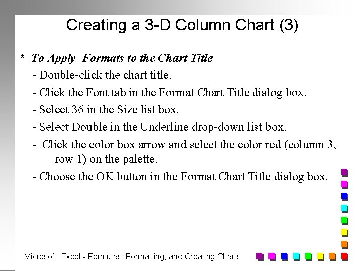
Creating a 3 -D Column Chart (3) * To Apply Formats to the Chart Title - Double-click the chart title. - Click the Font tab in the Format Chart Title dialog box. - Select 36 in the Size list box. - Select Double in the Underline drop-down list box. - Click the color box arrow and select the color red (column 3, row 1) on the palette. - Choose the OK button in the Format Chart Title dialog box. Microsoft Excel - Formulas, Formatting, and Creating Charts

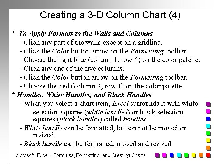
Creating a 3 -D Column Chart (4) * To Apply Formats to the Walls and Columns - Click any part of the walls except on a gridline. - Click the Color button arrow on the Formatting toolbar - Choose the light blue (column 1, row 5) on the color palette. - Click any one of the five columns. - Click the Color button arrow on the Formatting toolbar. - Choose the red (column 3, row 1) on the color palette. * Handles, White Handles, and Black Handles - When you select a chart item, Excel surrounds it with white selection squares (white handles) or black selection squares (black handles) called handles. - White handle can be formatted, but cannot be moved or resized. - Black handle can be formatted, moved and resized. Microsoft Excel - Formulas, Formatting, and Creating Charts

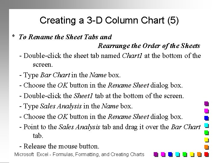
Creating a 3 -D Column Chart (5) * To Rename the Sheet Tabs and Rearrange the Order of the Sheets - Double-click the sheet tab named Chart 1 at the bottom of the screen. - Type Bar Chart in the Name box. - Choose the OK button in the Rename Sheet dialog box. - Double-click the Sheet 1 tab at the bottom of the screen. - Type Sales Analysis in the Name box. - Choose the OK button in the Rename Sheet dialog box. - Point to the Sales Analysis tab and drag it over the Bar Chart tab. - Release the mouse button. Microsoft Excel - Formulas, Formatting, and Creating Charts

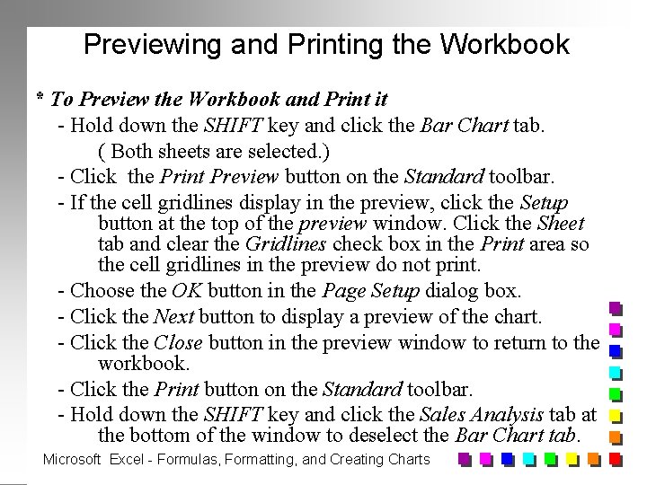
Previewing and Printing the Workbook * To Preview the Workbook and Print it - Hold down the SHIFT key and click the Bar Chart tab. ( Both sheets are selected. ) - Click the Print Preview button on the Standard toolbar. - If the cell gridlines display in the preview, click the Setup button at the top of the preview window. Click the Sheet tab and clear the Gridlines check box in the Print area so the cell gridlines in the preview do not print. - Choose the OK button in the Page Setup dialog box. - Click the Next button to display a preview of the chart. - Click the Close button in the preview window to return to the workbook. - Click the Print button on the Standard toolbar. - Hold down the SHIFT key and click the Sales Analysis tab at the bottom of the window to deselect the Bar Chart tab. Microsoft Excel - Formulas, Formatting, and Creating Charts

Print a Section of the Worksheet * To Print a Section of the Worksheet - Select the range A 3: C 8. - Choose the Print command from the File menu. - Click the Selection option button in the Print dialog box. - Choose the OK Button in the Print dialog box. Microsoft Excel - Formulas, Formatting, and Creating Charts

Display an Printing the Formulas in the Worksheet * To Display the Formulas in the Worksheet - Press CTRL + ` (Single quotation mark next to 1 key). ( Excel changes the display from values to formulas. ) - Choose the Page Setup command from the File menu. - From the Page Setup dialog box, click the Page tab. - Select the Landscape option and Fit to option to fit the wide printout on one page in landscape orientation. ( Portrait orientation- width of 8. 5 inches Landscape orientation- width of 11 inches) - Choose the OK button from the Page Setup dialog box. - Click the Print tool on the Standard toolbar. - When you are finished with the formulas version, press CTRL + `(single quotation mark next to 1 key) to display the values version. Microsoft Excel - Formulas, Formatting, and Creating Charts