L 12 Population Genomics Allele frequencies and Allele

L 12. Population Genomics

Allele frequencies and Allele Frequency Spectrum

Population and the hidden genealogy 0 1 2 3 4 5 6 7 8 9 4 0 6 7, 8 9 2 1, 3, 5 1 0 0 0 1 1 0 0 0 0 1 1 0 0 0 0 0 1 1 0 1 0 1 0 0 2 1 1 1 3 1 2 5

The Population sample • • • Mutations are constantly arising in a population Each mutation is eventually lost, either due to elimination, or due to fixation The rate at which this happens depends upon the selective pressure on the mutation. – • Selection: the rate at which a carrier is chosen as a parent. Under non-selective forces, the population is likely to be in equilibrium of various sorts

Allele Frequency Spectrum 0 0 1 0 1 1 1 0 0 0 0 0 1 1 1 0 0 0 1 1 0 1 0 0 0 0 1 1 0 0 1 0 1 0 0 0 1 1 0 0 0 0 1 0 4 3 2 1 1 Frequency 1 2 3 4 5 6 7 Count 1 0 0 0 1 0 1 0 0 1 1 0 2 1 3 2 1 2 7 1 5 6 3 4 1 Scaled Count Frequency 4 6 6 4 5 6 7 1 2 3 4 5 6 7

Scaled SFS of Neutral Evolution Scaled (Normalized) Count Outside of syllabus Frequenc y (Fu, 1995) * average of 500 simulated population samples

THE HARDY-WEINBERG EQUILIBRIUM AND ITS APPLICATIONS

Hardy-Weinberg principle Time (generations) Given: • • A Population of diploid individuals and a locus with alleles, A & a 3 Genotypes: AA, Aa, aa Q: Will the frequency of alleles and genotypes remain constant from generation to generation? a

To the Editor of Science: I am reluctant to intrude in a discussion concerning matters of which I have no expert knowledge, and I should have expected the very simple point which I wish to make to have been familiar to biologists. However, some remarks of Mr. Udny Yule, to which Mr. R. C. Punnett has called my attention, suggest that it may still be worth making. . . ………. A little mathematics of the multiplication-table type is enough to show …. the condition for this is q 2 = pr. And since q 12 = p 1 r 1, whatever the values of p, q, and r may be, the distribution will in any case continue unchanged after the second generation

Hardy Weinberg equilibrium Suppose, Pr(A)=p, and Pr(a)=1 p=q If certain assumptions are met • • Large, diploid, population Discrete generations Random mating No selection, … Aa Then, in every generation AA aa

Hardy-Weinberg principle • In the next generation Time (generations) A a

Hardy Weinberg: Generalization • Multiple alleles with frequencies – • By HW, Multiple loci?

APPLICATIONS OF THE HARDY-WEINBERG EQUILIBRIUM

Hardy Weinberg: Implications • It is observed that 1 in 10, 000 Caucasians have the disease phenylketonuria. The disease mutation(s) are recessive. What fraction of the population carries the mutation?

Hardy Weinberg: Implications • Males are 100 times more likely to have the ‘red’ type of color blindness than females. Why?

Hardy Weinberg: Implications • Individuals homozygous for S have the sickle-cell disease. In an experiment, the ratios A/A: A/S: S/S were 9365: 2993: 29. Is HWE violated? Is there a reason for this violation?

A modern example • B/B A/B • A/A SNP-chips can give us the genotype at each site based on hybridization. Plot the 3 genotypes at each locus on 3 separate horizontal lines. Genomic location B/B A/B Zoomed Out Picture A/A Genomic location

A modern example of HW application • • • SNP-chips can give us the allelic value at each polymorphic site based on hybridization. What is peculiar in the picture? What is your conclusion?

Hardy Weinberg: Quiz • The so called `bread wheat' is hexaploid (6 copies of each chromosome). Consider a locus with 4 allelic values (a; b; c; d ) with frequencies 0: 5; 0: 25; 0: 1, respectively. 1. 2. 3. • • Compute the number of distinct possible genotypes. Compute the expected number of occurrences of the genotype ab 3 c 2 in a sample of 10, 000 individuals, assuming HW equilibrium holds Generalize part (a) to compute the number of distinct genotypes given a ploidy of n (n copies of each chromosome) and m alleles A group of individuals In New York City was genotyped. Would you be surprised if HWE was violated? Males are 100 times more likely to have the ‘red’ type of color blindness than females. Why?

The power of HWE • • • Violation of HWE is common in nature Non-HWE implies that some assumption is violated Figuring out the violated assumption leads to biological insight

Hardy Weinberg: Quiz • The so called `bread wheat' is hexaploid (6 copies of each chromosome). Consider a locus with 4 allelic values (a; b; c; d ) with frequencies 0: 5; 0: 25; 0: 1, respectively. 1. 2. 3. • • Compute the number of distinct possible genotypes. Compute the expected number of occurrences of the genotype ab 3 c 2 in a sample of 10, 000 individuals, assuming HW equilibrium holds Generalize part (a) to compute the number of distinct genotypes given a ploidy of n (n copies of each chromosome) and m alleles A group of individuals In New York City was genotyped. Would you be surprised if HWE was violated? Males are 100 times more likely to have the ‘red’ type of color blindness than females. Why?

Perfect phylogeny

Scenario without recombination • • • The mt. DNA is identified directly from the mother Males inherit the y-chromosome directly from their father The genealogical relationship of these chromosomes does not involve recombination – – • Each individual has a single parent in the previous generation The genealogy is expressed as a tree. This principle can be used to track ancestry and migration history of a population CSE 280 Vineet Bafna

Phylogeny 0100 0011 1000 • Recall that we often study a population in the form of a SNP matrix – – – Rows correspond to individuals (or individual chromosomes), columns correspond to SNPs The matrix is binary (why? ) The underlying genealogy is hidden. If the span is large, the genealogy is not a tree any more. Why?

Reconstructing Perfect Phylogeny • • Input: SNP matrix M (n rows, m columns/sites/mutations) Output: a tree with the following properties – – – Rows correspond to leaf nodes We add mutations to edges each edge labeled with i splits the individuals into two subsets. • • i Individuals with a 1 in column i Individuals with a 0 in column i 1 in position i 0 in position i CSE 280 Vineet Bafna

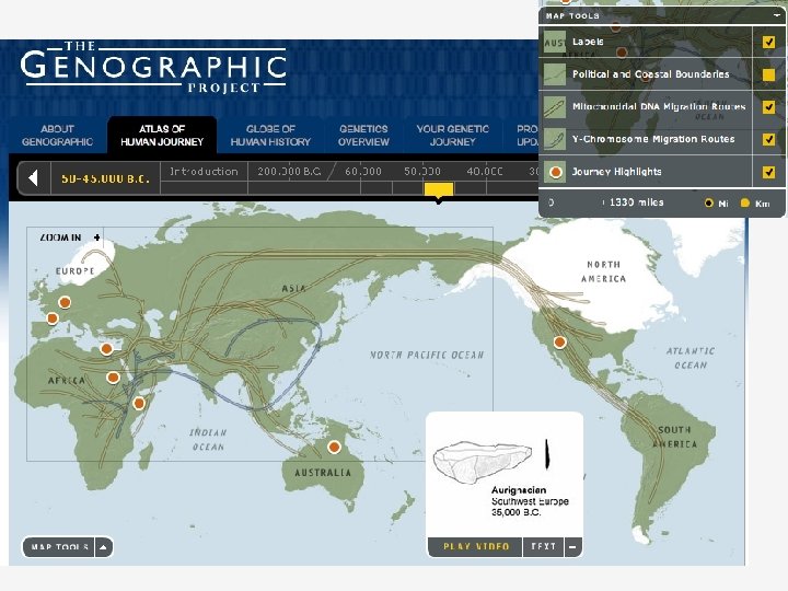
Reconstructing perfect phylogeny 2 6 3 1 7 4 5 8 12345678 01000000 00110110 00110100 00110000 100010001001 • Each mutation can be labeled by the column number Goal is to reconstruct the phylogeny • genographic atlas •

An algorithm for constructing a perfect phylogeny • • We will consider the case where 0 is the ancestral state, and 1 is the mutated state. This will be fixed later. In any tree, each node (except the root) has a single parent. – • • It is sufficient to construct a parent for every node. In each step, we add a column and refine some of the nodes containing multiple children. Stop if all columns have been considered. CSE 280 Vineet Bafna

Columns • • Define i 0: taxa (individuals) with a 0 at the i’th column Define i 1: taxa (individuals) with a 1 at the i’th column CSE 280 Vineet Bafna

Inclusion Property • For any pair of columns i, j, one of the following holds – – – • • i 1 j 1 = For any pair of columns i, j – i < j if and only if i 1 j 1 Note that if i<j then the edge containing i is an ancestor of the edge containing j CSE 280 Vineet Bafna i j

Perfect Phylogeny via Example r 12345 A 11000 B 00100 C 11010 D 00101 E 10000 A B C D Initially, there is a single clade r, and each node has r as its parent CSE 280 Vineet Bafna E

Sort columns • • Sort columns according to the inclusion property (note that the columns are already sorted here). This can be achieved by considering the columns as binary representations of numbers (most significant bit in row 1) and sorting in decreasing order CSE 280 Vineet Bafna 12345 A 11000 B 00100 C 11010 D 00101 E 10000

Add first column • In adding column i – – 12345 A 11000 B 00100 C 11010 D 00101 E 10000 Check each individual and decide which side you belong. Finally add a node if you can resolve a clade r u A CSE 280 Vineet Bafna C E B D

Adding other columns • Add other columns on edges using the ordering property 12345 A 11000 B 00100 C 11010 D 00101 E 10000 r 1 3 2 E Vineet Bafna B 4 C CSE 280 5 D A

Unrooted case • • Important point is that the perfect phylogeny condition does not change when you interchange 1 s and 0 s at a column. Alg (Unrooted) – – – • Switch the values in each column, so that 0 is the majority element. Apply the algorithm for the rooted case. Relabel columns and individuals. Show that this is a correct algorithm. CSE 280 Vineet Bafna

Unrooted perfect phylogeny • • • We transform matrix M to a 0 -major matrix M 0. if M 0 has a directed perfect phylogeny, M has a perfect phylogeny. If M has a perfect phylogeny, does M 0 have a directed perfect phylogeny?

Unrooted case • Theorem: If M has a perfect phylogeny, there exists a relabeling, and a perfect phylogeny s. t. – – – CSE 280 Root is all 0 s For any SNP (column), #1 s <= #0 s All edges are mutated 0 1 Vineet Bafna

Proof • • Consider the perfect phylogeny of M. Find the center: none of the clades has greater than n/2 nodes. – • • Is this always possible? Root at one of the 3 edges of the center, and direct all mutations from 0 1 away from the root. QED If theorem is correct, then simply relabeling all columns so that the majority element is 0 is sufficient. CSE 280 Vineet Bafna

Finding the center

‘Homework’ Problems • • What if there is missing data? (An entry that can be 0 or 1)? What if there are recurrent mutations? CSE 280 Vineet Bafna

The Neandertal genome, 2009

Introgression with Neanderthals Science News We can predict when the introgression event happened, and what regions of the genome have Neanderthal heritage.

Linkage Disequilibrium

Quiz • Recall that a SNP data-set is a ‘binary’ matrix. – – • Rows are individual (chromosomes) Columns are alleles at a specific locus Suppose you have 2 SNP datasets of a contiguous genomic region but no other information – – – One from an African population, and one from a European Population. Can you tell which is which? How long does the genomic region have to be?

Linkage (Dis)-equilibrium (LD) • • • Consider sites A &B Case 1: No recombination Each new individual chromosome chooses a parent from the existing ‘haplotype’ A 0 0 1 1 1 B 1 1 0 0 0 0

Linkage (Dis)-equilibrium (LD) • • • Consider sites A &B Case 2: diploidy and recombination Each new individual chooses a parent from the existing alleles A 0 0 1 1 1 B 1 1 0 0 0 1

Linkage (Dis)-equilibrium (LD) • • • Consider sites A &B Case 1: No recombination Each new individual chooses a parent from the existing ‘haplotype’ – Pr[A, B=0, 1] = 0. 25 • Linkage disequilibrium Case 2: Extensive recombination Each new individual simply chooses and allele from either site – Pr[A, B=(0, 1)]=0. 125 • Linkage equilibrium A 0 0 1 1 B 1 1 0 0 0

LD • In the absence of recombination, – – • Correlation between columns The joint probability Pr[A=a, B=b] is different from P(a)P(b) With extensive recombination – Pr(a, b)=P(a)P(b)

Measures of LD • • Consider two bi-allelic sites with alleles marked with 0 and 1 Define – – • • P 00 = Pr[Allele 0 in locus 1, and 0 in locus 2] P 0* = Pr[Allele 0 in locus 1] Linkage equilibrium if P 00 = P 0* P*0 The D-measure of LD – D = (P 00 - P 0* P*0) = -(P 01 - P 0* P*1) = …

Other measures of LD • D’ is obtained by dividing D by the largest possible value – – Suppose D = (P 00 - P 0* P*0) >0. Then the maximum value of Dmax= min{P 0* P*1, P 1* P*0} If D<0, then maximum value is max{-P 0* P*0, -P 1* P*1} D’ = D/ Dmax 0 0 1 D -D -D D Site 1 1 Site 2

A STATISTICAL DIGRESSION

Normal distribution and Z-scores μ σ • • x The p-value of x can be computed by looking up a table for N(μ, σ). Also, the Z-score can be computed as Z=(x-μ)/σ – Z is distributed according to N(0, 1)

Chi-Square distribution • Think of a chi-square distribution as the square of a Normal distribution.

Chi-square test • • • Testing for correlation between two variables. If O = observed value, E = expected value, then the following behaves like a chi-square distributed variable The sum of chi-square variables is also chisquare distributed.

Other measures of LD • • D’ is obtained by dividing D by the largest possible value – Ex: D’ = abs(P 11 - P 1* P*1)/ Dmax = D/(P 1* P 0* P*1 P*0)1/2 Let N be the number of individuals Show that 2 N is the 2 statistic between the two sites 0 0 P 00 N Site 1 1 Site 2 1 P 0*N

Digression: The χ2 test • • 0 1 0 O 1 O 2 1 O 3 O 4 The statistic behaves like a χ2 distribution (sum of squares of normal variables). A p-value can be computed directly

Observed and expected Site 1 0 1 P 00 N P 01 N P 0*P*0 N P 0*P*1 N 1 P 10 N P 11 N P 1*P*0 N P 1*P*1 N 0 0 1 • = D/(P 1* P 0* P*1 P*0)1/2 • Verify that 2 N is the 2 statistic between the two sites

LD over time and distance • • The number of recombination events between two sites, can be assumed to be Poisson distributed. Let r denote the recombination rate between two adjacent sites r = # crossovers per bp per generation The recombination rate between two sites l apart is rl

LD over time • Decay in LD – – – Let D(t) = LD at time t between two sites r’=lr P(t)00 = (1 -r’) P(t-1)00 + r’ P(t-1)0* P(t-1)*0 D(t) = P(t)00 - P(t)0* P(t)*0 = P(t)00 - P(t-1)0* P(t-1)*0 (Why? ) D(t) =(1 -r’) D(t-1) =(1 -r’)t D(0)

LD over distance • Assumption – – • • Recombination rate increases linearly with distance and time LD decays exponentially. The assumption is reasonable, but recombination rates vary from region to region, adding to complexity This simple fact is the basis of disease association mapping.

LD and disease mapping • • • Consider a mutation that is causal for a disease. The goal of disease gene mapping is to discover which gene (locus) carries the mutation. Consider every polymorphism, and check: – – • There might be too many polymorphisms Multiple mutations (even at a single locus) that lead to the same disease Instead, consider a dense sample of polymorphisms that span the genome

LD can be used to map disease genes LD D N N D D N • • 0 1 1 0 0 1 LD decays with distance from the disease allele. By plotting LD, one can short list the region containing the disease gene.

• 269 individuals – – • 90 Yorubans 90 Europeans (CEPH) 44 Japanese 45 Chinese ~1 M SNPs

Haplotype blocks • It was found that recombination rates vary across the genome – • • How can the recombination rate be measured? In regions with low recombination, you expect to see long haplotypes that are conserved. Why? Typically, haplotype blocks do not span recombination hot-spots

19 q 13

Long haplotypes • • • Chr 2 region with high r 2 value (implies little/no recombination) History/Genealogy can be explained by a tree ( a perfect phylogeny) Large haplotypes with high frequency are observed

LD variation across populations • LD is maintained upto 60 kb in swedish population, 6 kb in Yoruban population Reich et al. Nature 411, 199 -204(10 May 2001)

Population specific recombination • • D’ was used as the measure between SNP pairs were classified in one of the following – – – • • Strong LD Strong evidence for recombination Others (13% of cases) Plot shows fraction of pairs with strong recombination (low LD) This roughly favors out-ofafrica. A Coalescent simulation can help give confidence values on this. Gabriel et al. , Science 2002

Introgression

Time of introgression

Introgression • • Consider SNPs at genetic distance x (#crossovers per generation) How will the introgressed SNPs behave differently from non-introgressed SNPs? Can we use them to get at time of introgression?

LD over time and distance • • • The number of recombination events between two sites, can be assumed to be Poisson distributed. Let x denote the recombination rate between two adjacent sites x = # crossovers in the region per meiosis

Decay of LD with time, and distance • • • S(x) all SNP pairs at genetic distance x. Compute ‘Average LD’ value If the genetic distance is correct, this can be used to give an estimate of the age of the SNP.

LD over time • Decay in LD – – CSE 280 Let D(t) = LD at time t between two sites P(t)00 = (1 -x) P(t-1)00 + x P(t-1)0* P(t-1)*0 D(t) = P(t)00 - P(t)0* P(t)*0 = P(t)00 - P(t-1)0* P(t-1)*0 (Why? ) D(t) =(1 -x) D(t-1) =(1 -x)t D(0) Vineet Bafna

Recent versus ancient SNPs • Recent origin (t is smaller) • Ancient origin (t is larger)

Figure 1. Linkage disequilibrium patterns expected due to recent gene flow and ancient structure. Sankararaman S, Patterson N, Li H, Pääbo S, Reich D (2012) The Date of Interbreeding between Neandertals and Modern Humans. PLo. S Genet 8(10): e 1002947. doi: 10. 1371/journal. pgen. 1002947 http: //127. 0. 0. 1: 8081/plosgenetics/article? id=info: doi/10. 1371/journal. pgen. 1002947

Figure 2. Classes of demographic models relating Africans (Y), Europeans (E), and Neandertals (N). Sankararaman S, Patterson N, Li H, Pääbo S, Reich D (2012) The Date of Interbreeding between Neandertals and Modern Humans. PLo. S Genet 8(10): e 1002947. doi: 10. 1371/journal. pgen. 1002947 http: //127. 0. 0. 1: 8081/plosgenetics/article? id=info: doi/10. 1371/journal. pgen. 1002947

Table 1. Estimates of the time of gene flow for different demographic models and mutation rates as well as different ascertainments. Sankararaman S, Patterson N, Li H, Pääbo S, Reich D (2012) The Date of Interbreeding between Neandertals and Modern Humans. PLo. S Genet 8(10): e 1002947. doi: 10. 1371/journal. pgen. 1002947 http: //127. 0. 0. 1: 8081/plosgenetics/article? id=info: doi/10. 1371/journal. pgen. 1002947