KULIAH X EXTERNAL INCOMPRESSIBLE VISCOUS FLOW Nazaruddin Sinaga

KULIAH X EXTERNAL INCOMPRESSIBLE VISCOUS FLOW Nazaruddin Sinaga Free Powerpoint Templates Page 1

Main Topics The Boundary-Layer Concept Boundary-Layer Thickness Laminar Flat-Plate Boundary Layer: Exact Solution Momentum Integral Equation Use of the Momentum Equation for Flow with Zero Pressure Gradient • Pressure Gradients in Boundary-Layer Flow • Drag • Lift • • •

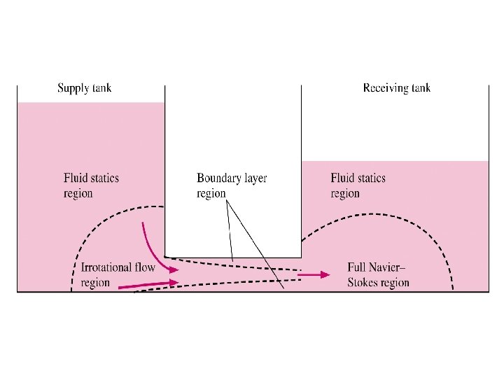
The Boundary-Layer Concept

The Boundary-Layer Concept

Boundary Layer Thickness

Boundary Layer Thickness • Disturbance Thickness, where ü Displacement Thickness, d* ü Momentum Thickness, q

Boundary Layer Laws 1. The velocity is zero at the wall (u = 0 at y = 0) 2. The velocity is a maximum at the top of the layer (u = um at = ) 3. The gradient of BL is zero at the top of the layer (du/dy = 0 at y = ) 4. The gradient is constant at the wall (du/dy = C at y = 0) 5. Following from (4): (d 2 u/dy 2 = 0 at y = 0)

Navier-Stokes Equation Cartesian Coordinates Continuity X-momentum Y-momentum Z-momentum

Laminar Flat-Plate Boundary Layer: Exact Solution • Governing Equations • For incompresible steady 2 D cases:

Laminar Flat-Plate Boundary Layer: Exact Solution • Boundary Conditions

Laminar Flat-Plate Boundary Layer: Exact Solution • Equations are Coupled, Nonlinear, Partial Differential Equations • Blassius Solution: – Transform to single, higher-order, nonlinear, ordinary differential equation

Boundary Layer Procedure • Before defining and * and are there analytical solutions to the BL equations? – Unfortunately, NO • Blasius Similarity Solution boundary layer on a flat plate, constant edge velocity, zero external pressure gradient

Blasius Similarity Solution • Blasius introduced similarity variables • This reduces the BLE to • This ODE can be solved using Runge. Kutta technique • Result is a BL profile which holds at every station along the flat plate

Blasius Similarity Solution

Blasius Similarity Solution • Boundary layer thickness can be computed by assuming that corresponds to point where U/Ue = 0. 990. At this point, = 4. 91, therefore Recall • Wall shear stress w and friction coefficient Cf, x can be directly related to Blasius solution

Displacement Thickness • Displacement thickness * is the imaginary increase in thickness of the wall (or body), as seen by the outer flow, and is due to the effect of a growing BL. • Expression for * is based upon control volume analysis of conservation of mass • Blasius profile for laminar BL can be integrated to give ( 1/3 of )

Momentum Thickness • Momentum thickness is another measure of boundary layer thickness. • Defined as the loss of momentum flux per unit width divided by U 2 due to the presence of the growing BL. • Derived using CV analysis. for Blasius solution, identical to Cf, x

Turbulent Boundary Layer Black lines: instantaneous Pink line: time-averaged Illustration of unsteadiness of a turbulent BL Comparison of laminar and turbulent BL profiles
![Turbulent Boundary Layer • All BL variables [U(y), , *, ] are determined empirically.](http://slidetodoc.com/presentation_image_h2/e6f1667d6280b87e5d7ff8c8f4fc8318/image-26.jpg "Turbulent Boundary Layer • All BL variables [U(y), , *, ] are determined empirically.")
Turbulent Boundary Layer • All BL variables [U(y), , *, ] are determined empirically. • One common empirical approximation for the time-averaged velocity profile is the oneseventh-power law

• Results of Numerical Analysis
 Solution")
Momentum Integral Equation • Provides Approximate Alternative to Exact (Blassius) Solution

Momentum Integral Equation is used to estimate the boundary-layer thickness as a function of x: 1. Obtain a first approximation to the freestream velocity distribution, U(x). The pressure in the boundary layer is related to the freestream velocity, U(x), using the Bernoulli equation 2. Assume a reasonable velocity-profile shape inside the boundary layer 3. Derive an expression for tw using the results obtained from item 2

Use of the Momentum Equation for Flow with Zero Pressure Gradient • Simplify Momentum Integral Equation (Item 1) ü The Momentum Integral Equation becomes

Use of the Momentum Equation for Flow with Zero Pressure Gradient Laminar Flow • – Example: Assume a Polynomial Velocity Profile (Item 2) • The wall shear stress tw is then (Item 3)

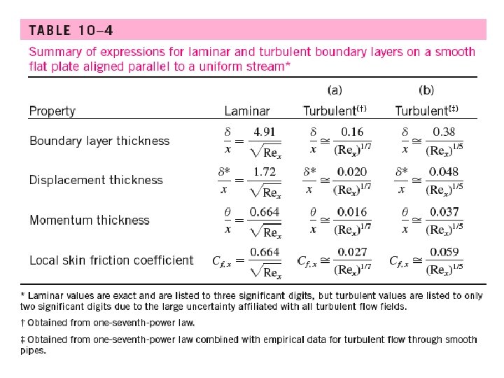
Use of the Momentum Equation for Flow with Zero Pressure Gradient • Laminar Flow Results (Polynomial Velocity Profile) Compare to Exact (Blassius) results!

Use of the Momentum Equation for Flow with Zero Pressure Gradient • Turbulent Flow – Example: 1/7 -Power Law Profile (Item 2)

Use of the Momentum Equation for Flow with Zero Pressure Gradient • Turbulent Flow Results (1/7 -Power Law Profile)

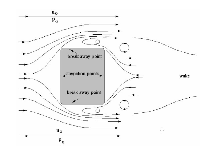
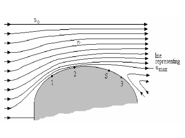
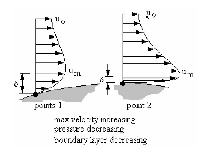
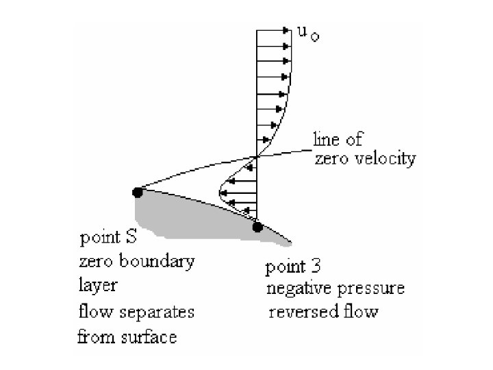
Pressure Gradients in Boundary-Layer Flow

DRAG AND LIFT • Fluid dynamic forces are due to pressure and viscous forces acting on the body surface. • Drag: component parallel to flow direction. • Lift: component normal to flow direction.

Drag and Lift • Lift and drag forces can be found by integrating pressure and wall-shear stress.

Drag and Lift • In addition to geometry, lift FL and drag FD forces are a function of density and velocity V. • Dimensional analysis gives 2 dimensionless parameters: lift and drag coefficients. • Area A can be frontal area (drag applications), planform area (wing aerodynamics), or wettedsurface area (ship hydrodynamics).

Drag • Drag Coefficient with or

Drag • Pure Friction Drag: Flat Plate Parallel to the Flow • Pure Pressure Drag: Flat Plate Perpendicular to the Flow • Friction and Pressure Drag: Flow over a Sphere and Cylinder • Streamlining

Drag • Flow over a Flat Plate Parallel to the Flow: Friction Drag Boundary Layer can be 100% laminar, partly laminar and partly turbulent, or essentially 100% turbulent; hence several different drag coefficients are available
")
Drag • Flow over a Flat Plate Parallel to the Flow: Friction Drag (Continued) Laminar BL: Turbulent BL: … plus others for transitional flow

Drag Coefficient 0, 140 0, 120 0, 100 CD Laminar 0, 080 CD Turbulen 0, 060 0, 040 0, 020 0, 000 1 E+02 1 E+03 1 E+04 1 E+05 1 E+06 1 E+07 1 E+08 1 E+09

Drag • Flow over a Flat Plate Perpendicular to the Flow: Pressure Drag coefficients are usually obtained empirically
")
Drag • Flow over a Flat Plate Perpendicular to the Flow: Pressure Drag (Continued)

Drag • Flow over a Sphere : Friction and Pressure Drag

Drag • Flow over a Cylinder: Friction and Pressure Drag

Streamlining • Used to Reduce Wake and Pressure Drag

Lift • Mostly applies to Airfoils Note: Based on planform area Ap

Lift • Examples: NACA 23015; NACA 662 -215

Lift • Induced Drag
 Reduction in Effective Angle of Attack: Finite Wing Drag")
Lift • Induced Drag (Continued) Reduction in Effective Angle of Attack: Finite Wing Drag Coefficient:
")
Lift • Induced Drag (Continued)

Fluid Dynamic Forces and Moments Ships in waves present one of the most difficult 6 DOF problems. Airplane in level steady flight: drag = thrust and lift = weight.

Example: Automobile Drag Scion XB Porsche 911 CD = 1. 0, A = 25 ft 2, CDA = 25 ft 2 CD = 0. 28, A = 10 ft 2, CDA = 2. 8 ft 2 • Drag force FD=1/2 V 2(CDA) will be ~ 10 times larger for Scion XB • Source is large CD and large projected area • Power consumption P = FDV =1/2 V 3(CDA) for both scales with V 3!

Drag and Lift • For applications such as tapered wings, CL and CD may be a function of span location. For these applications, a local CL, x and CD, x are introduced and the total lift and drag is determined by integration over the span L

Friction and Pressure Drag Friction drag • Fluid dynamic forces are comprised of pressure and friction effects. • Often useful to decompose, – FD = FD, friction + FD, pressure – CD = CD, friction + CD, pressure Pressure drag Friction & pressure drag • This forms the basis of ship model testing where it is assumed that – CD, pressure = f(Fr) – CD, friction = f(Re)

Streamlining • Streamlining reduces drag by reducing FD, pressure, at the cost of increasing wetted surface area and FD, friction. • Goal is to eliminate flow separation and minimize total drag FD • Also improves structural acoustics since separation and vortex shedding can excite structural modes.

Streamlining

Streamlining via Active Flow Control • Pneumatic controls for blowing air from slots: reduces drag, improves fuel economy for heavy trucks (Dr. Robert Englar, Georgia Tech Research Institute).

CD of Common Geometries • For many geometries, total drag CD is constant for Re > 104 • CD can be very dependent upon orientation of body. • As a crude approximation, superposition can be used to add CD from various components of a system to obtain overall drag. However, there is no mathematical reason (e. g. , linear PDE's) for the success of doing this.

CD of Common Geometries

CD of Common Geometries

CD of Common Geometries

Flat Plate Drag • Drag on flat plate is solely due to friction created by laminar, transitional, and turbulent boundary layers.

Flat Plate Drag • Local friction coefficient – Laminar: – Turbulent: • Average friction coefficient – Laminar: – Turbulent: For some cases, plate is long enough for turbulent flow, but not long enough to neglect laminar portion

Effect of Roughness • Similar to Moody Chart for pipe flow • Laminar flow unaffected by roughness • Turbulent flow significantly affected: Cf can increase by 7 x for a given Re

Cylinder and Sphere Drag

Cylinder and Sphere Drag • Flow is strong function of Re. • Wake narrows for turbulent flow since TBL (turbulent boundary layer) is more resistant to separation due to adverse pressure gradient. • sep, lam ≈ 80º • sep, turb ≈ 140º

Effect of Surface Roughness
 perpendicular")
Lift • Lift is the net force (due to pressure and viscous forces) perpendicular to flow direction. • Lift coefficient • A=bc is the planform area

Computing Lift • Potential-flow approximation gives accurate CL for angles of attack below stall: boundary layer can be neglected. • Thin-foil theory: superposition of uniform stream and vortices on mean camber line. • Java-applet panel codes available online: http: //www. aa. nps. navy. mil/~jones/online_t ools/panel 2/ • Kutta condition required at trailing edge: fixes stagnation pt at TE.

Effect of Angle of Attack • Thin-foil theory shows that CL≈2 for < stall • Therefore, lift increases linearly with • Objective for most applications is to achieve maximum CL/CD ratio. • CD determined from wind-tunnel or CFD (BLE or NSE). • CL/CD increases (up to order 100) until stall.
")
Effect of Foil Shape • Thickness and camber influences pressure distribution (and load distribution) and location of flow separation. • Foil database compiled by Selig (UIUC) http: //www. aae. uiuc. ed u/m-selig/ads. html

Effect of Foil Shape • Figures from NPS airfoil java applet. • Color contours of pressure field • Streamlines through velocity field • Plot of surface pressure • Camber and thickness shown to have large impact on flow field.

End Effects of Wing Tips • Tip vortex created by leakage of flow from highpressure side to lowpressure side of wing. • Tip vortices from heavy aircraft persist far downstream and pose danger to light aircraft. Also sets takeoff and landing separation at busy airports.

End Effects of Wing Tips • Tip effects can be reduced by attaching endplates or winglets. • Trade-off between reducing induced drag and increasing friction drag. • Wing-tip feathers on some birds serve the same function.

Lift Generated by Spinning Superposition of Uniform stream + Doublet + Vortex

Lift Generated by Spinning • CL strongly depends on rate of rotation. • The effect of rate of rotation on CD is small. • Baseball, golf, soccer, tennis players utilize spin. • Lift generated by rotation is called The Magnus Effect.

The End Terima kasih Free Powerpoint Templates 81 Page 81

Derivation of the boundary layer equations II 82

Blassius exact solution I Boundary layer over a flat plate = Ue 1 Variable transformation: Wall boundary condition: , Stream function definition: , 83

Blassius exact solution II Boundary layer over a flat plate Ordinary differential equation Boundary conditions The analytical solution of the ordinary differential equation was obtained by Blasius using series expansions 84

Blassius exact solution III Boundary layer over a flat plate Solution Velocity along x 1 -direction: Velocity along x 2 -direction: Boundary layer thickness: Displacement thickness: Wall shear stress: 85

Blassius exact solution IV Boundary layer over a flat plate Solution 86

Von Karman integral momentum equation I Momentum conservation along x 1 -direction 87
 = pe(x 1) 88")
Von Karman integral momentum equation II Solution Considerations: p(x 1) = pe(x 1) 88

Approximate solutions I Linear, quadratic, cubic and sinusoidal velocity profiles 1. Assumption of a self-similar velocity profile U 1*= f (x 2*) 2. Specifications of the boundary conditions 3. Resolution of the Von Karman integral momentum equation 89

Approximate solutions II Example: quadratic velocity profiles Velocity profile General form + boundary conditions = velocity profile along x 1 -dir Von Karman integral momentum equation solution boundary layer thickness 90

Approximate solutions III Example: quadratic velocity profiles Displacement thickness: from the definition => Velocity along x 2 -direction from continuity equation Wall shear stress from => 91
- Slides: 91