KULIAH VIII IX MEKANIKA FLUIDA II Nazaruddin Sinaga

KULIAH VIII - IX MEKANIKA FLUIDA II Nazaruddin Sinaga Free Powerpoint Templates Page 1

Entrance Length 2

Shear stress and velocity distribution in pipe for laminar flow

Typical velocity and shear distributions in turbulent flow near a wall: (a) shear; (b) velocity. 4

Solution of Pipe Flow Problems • Single Path – Find Dp for a given L, D, and Q Ø Use energy equation directly – Find L for a given Dp, D, and Q Ø Use energy equation directly

Solution of Pipe Flow Problems • Single Path (Continued) – Find Q for a given Dp, L, and D 1. Manually iterate energy equation and friction factor formula to find V (or Q), or 2. Directly solve, simultaneously, energy equation and friction factor formula using (for example) Excel – Find D for a given Dp, L, and Q 1. Manually iterate energy equation and friction factor formula to find D, or 2. Directly solve, simultaneously, energy equation and friction factor formula using (for example) Excel

Example 1 § Water at 10 C is flowing at a rate of 0. 03 m 3/s through a pipe. The pipe has 150 -mm diameter, 500 m long, and the surface roughness is estimated at 0. 06 mm. Find the head loss and the pressure drop throughout the length of the pipe. Solution: § From Table 1. 3 (for water): = 1000 kg/m 3 and =1. 30 x 10 -3 N. s/m 2 V = Q/A and A= R 2 A = (0. 15/2)2 = 0. 01767 m 2 V = Q/A =0. 03/. 0. 01767 =1. 7 m/s Re = (1000 x 1. 7 x 0. 15)/(1. 30 x 10 -3) = 1. 96 x 105 > 2000 turbulent flow To find , use Moody Diagram with Re and relative roughness (k/D). k/D = 0. 06 x 10 -3/0. 15 = 4 x 10 -4 From Moody diagram, 0. 018 The head loss may be computed using the Darcy-Weisbach equation. The pressure drop along the pipe can be calculated using the relationship: ΔP= ghf = 1000 x 9. 81 x 8. 84 ΔP = 8. 67 x 104 Pa 7

Example 2 § Determine the energy loss that will occur as 0. 06 m 3/s water flows from a 40 -mm pipe diameter into a 100 -mm pipe diameter through a sudden expansion. Solution: § The head loss through a sudden enlargement is given by; Da/Db = 40/100 = 0. 4 From Table 6. 3: K = 0. 70 Thus, the head loss is 8

Example 3 § Calculate the head added by the pump when the water system shown below carries a discharge of 0. 27 m 3/s. If the efficiency of the pump is 80%, calculate the power input required by the pump to maintain the flow. 9

Solution: Applying Bernoulli equation between section 1 and 2 (1) P 1 = P 2 = Patm = 0 (atm) and V 1=V 2 0 Thus equation (1) reduces to: (2) HL 1 -2 = hf + hentrance + hbend + hexit From (2):

The velocity can be calculated using the continuity equation: Thus, the head added by the pump: Pin = 130. 117 Watt ≈ 130 k. W. Hp = 39. 3 m

EGL & HGL for a Pipe System • Energy equation • • All terms are in dimension of length (head, or energy per unit weight) HGL – Hydraulic Grade Line • EGL – Energy Grade Line • • EGL=HGL when V=0 (reservoir surface, etc. ) EGL slopes in the direction of flow

EGL & HGL for a Pipe System • A pump causes an abrupt rise in EGL (and HGL) since energy is introduced here

EGL & HGL for a Pipe System • A turbine causes an abrupt drop in EGL (and HGL) as energy is taken out • Gradual expansion increases turbine efficiency

EGL & HGL for a Pipe System • • When the flow passage changes diameter, the velocity changes so that the distance between the EGL and HGL changes When the pressure becomes 0, the HGL coincides with the system

EGL & HGL for a Pipe System • Abrupt expansion into reservoir causes a complete loss of kinetic energy there

EGL & HGL for a Pipe System • When HGL falls below the pipe the pressure is below atmospheric pressure

FLOW MEASUREMENT • Direct Methods – Examples: Accumulation in a Container; Positive Displacement Flowmeter • Restriction Flow Meters for Internal Flows – Examples: Orifice Plate; Flow Nozzle; Venturi; Laminar Flow Element

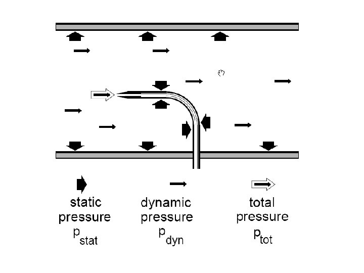
Definisi tekanan pada aliran di sekitar sayap

Flow Measurement • Linear Flow Meters – Examples: Float Meter (Rotameter); Turbine; Vortex; Electromagnetic; Magnetic; Ultrasonic Float-type variablearea flow meter

Flow Measurement • Linear Flow Meters – Examples: Float Meter (Rotameter); Turbine; Vortex; Electromagnetic; Magnetic; Ultrasonic Turbine flow meter

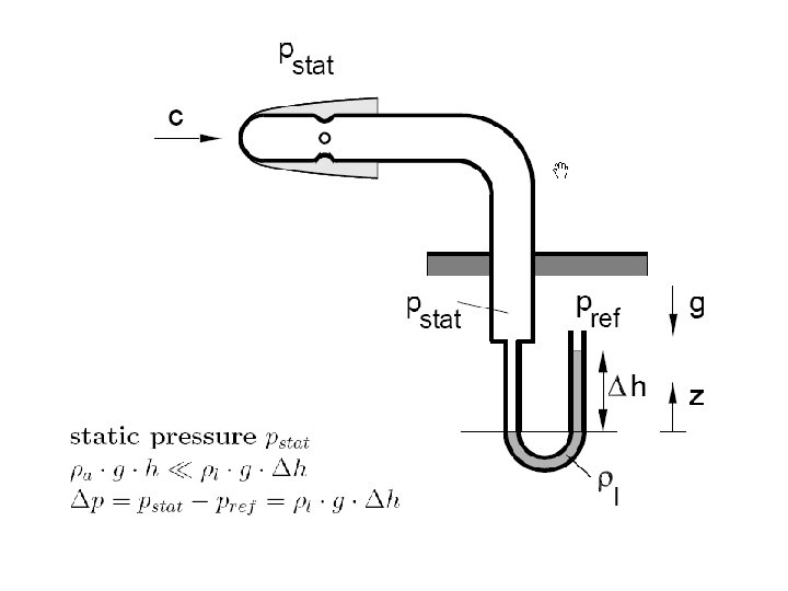
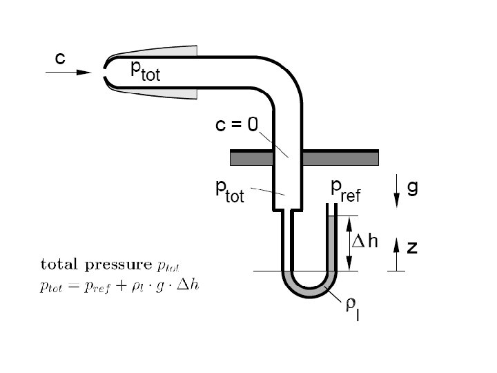
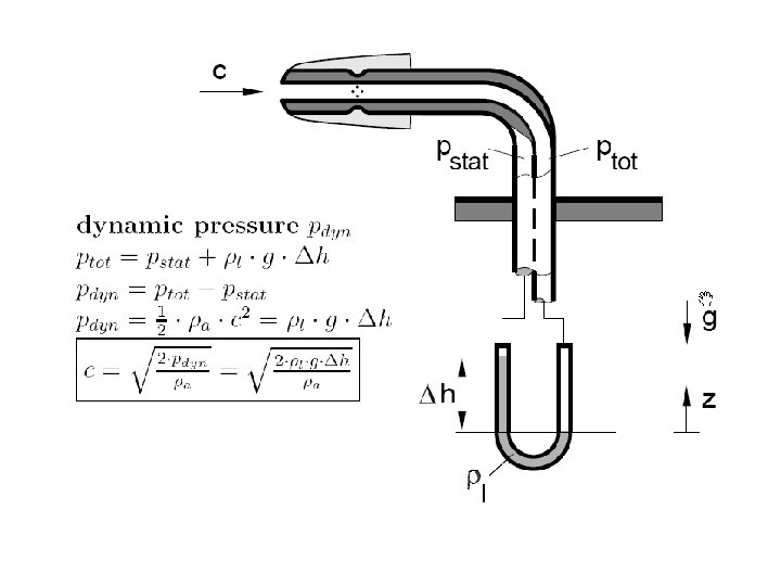
Flow Measurement • Traversing Methods – Examples: Pitot (or Pitot Static) Tube; Laser Doppler Anemometer

The measured stagnation pressure cannot of itself be used to determine the fluid velocity (airspeed in aviation). However, Bernoulli's equation states: Stagnation pressure = static pressure + dynamic pressure Which can also be written 30

Solving that for velocity we get: Note: The above equation applies only to incompressible fluid. where: § § V is fluid velocity; pt is stagnation or total pressure; ps is static pressure; and ρ is fluid density. 31

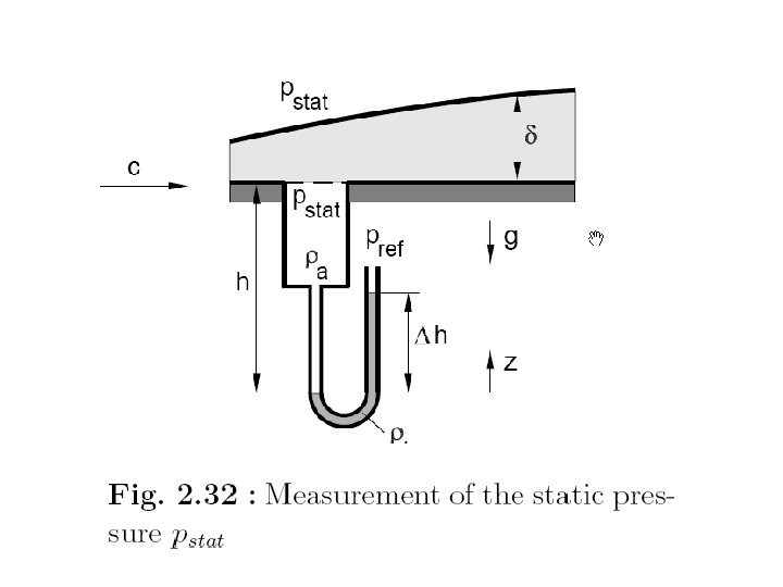
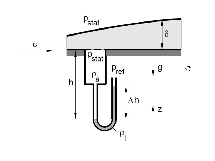
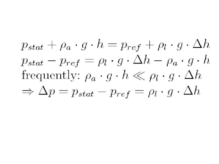
The value for the pressure drop p 2 – p 1 or Δp to Δh, the reading on the manometer: Δp = Δh(ρA-ρ)g Where: § ρA is the density of the fluid in the manometer § Δh is the manometer reading 32

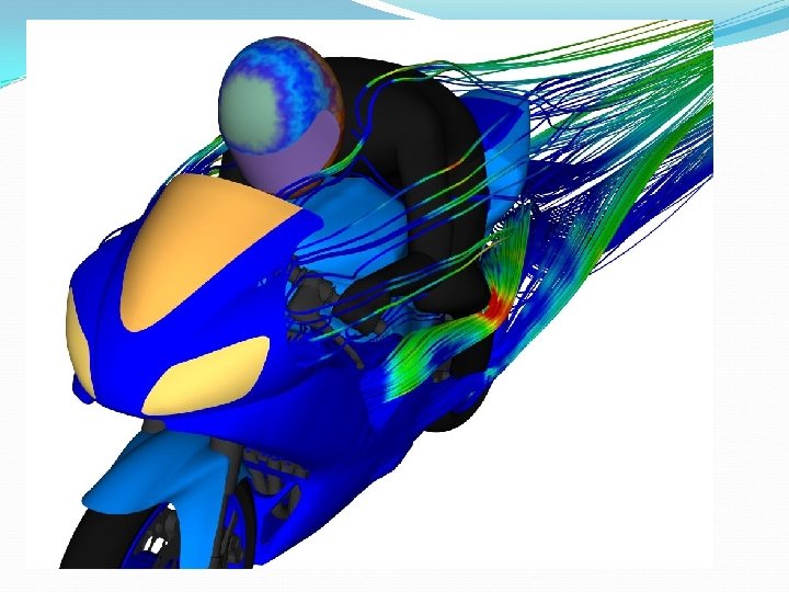
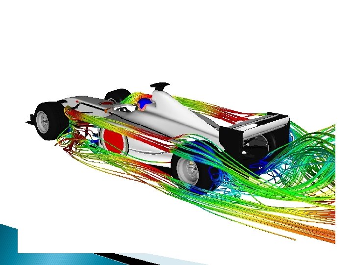
EXTERNAL INCOMPRESSIBLE VISCOUS FLOW

Main Topics The Boundary-Layer Concept Boundary-Layer Thickness Laminar Flat-Plate Boundary Layer: Exact Solution Momentum Integral Equation Use of the Momentum Equation for Flow with Zero Pressure Gradient • Pressure Gradients in Boundary-Layer Flow • Drag • Lift • • •

The Boundary-Layer Concept

The Boundary-Layer Concept

Boundary Layer Thickness

Boundary Layer Thickness • Disturbance Thickness, d where ü Displacement Thickness, d* ü Momentum Thickness, q

Boundary Layer Laws

Laminar Flat-Plate Boundary Layer: Exact Solution • Governing Equations

Laminar Flat-Plate Boundary Layer: Exact Solution • Boundary Conditions

Laminar Flat-Plate Boundary Layer: Exact Solution • Equations are Coupled, Nonlinear, Partial Differential Equations • Blassius Solution: – Transform to single, higher-order, nonlinear, ordinary differential equation

Laminar Flat-Plate Boundary Layer: Exact Solution • Results of Numerical Analysis

Momentum Integral Equation • Provides Approximate Alternative to Exact (Blassius) Solution

Momentum Integral Equation is used to estimate the boundary-layer thickness as a function of x: 1. Obtain a first approximation to the freestream velocity distribution, U(x). The pressure in the boundary layer is related to the freestream velocity, U(x), using the Bernoulli equation 2. Assume a reasonable velocity-profile shape inside the boundary layer 3. Derive an expression for tw using the results obtained from item 2

Use of the Momentum Equation for Flow with Zero Pressure Gradient • Simplify Momentum Integral Equation (Item 1) ü The Momentum Integral Equation becomes

Use of the Momentum Equation for Flow with Zero Pressure Gradient Laminar Flow • – Example: Assume a Polynomial Velocity Profile (Item 2) • The wall shear stress tw is then (Item 3)

Use of the Momentum Equation for Flow with Zero Pressure Gradient • Laminar Flow Results (Polynomial Velocity Profile) Compare to Exact (Blassius) results!

Use of the Momentum Equation for Flow with Zero Pressure Gradient • Turbulent Flow – Example: 1/7 -Power Law Profile (Item 2)

Use of the Momentum Equation for Flow with Zero Pressure Gradient • Turbulent Flow Results (1/7 -Power Law Profile)

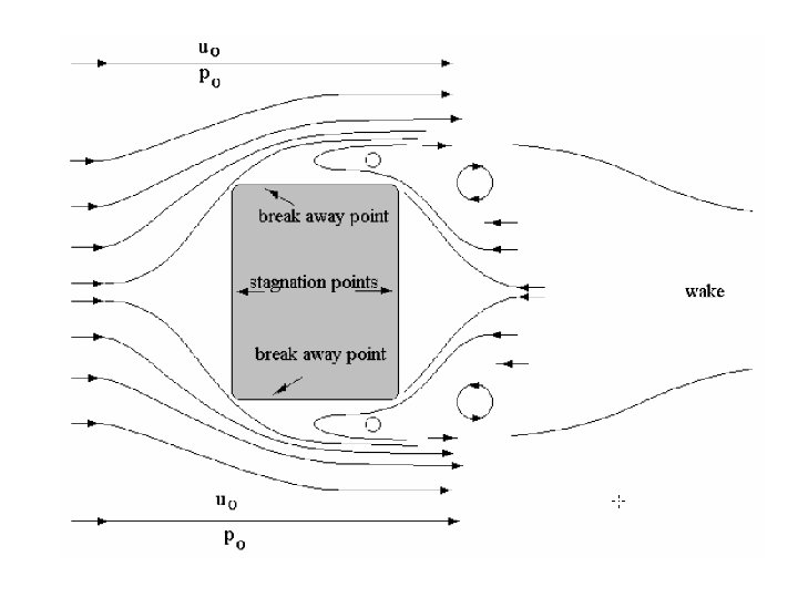
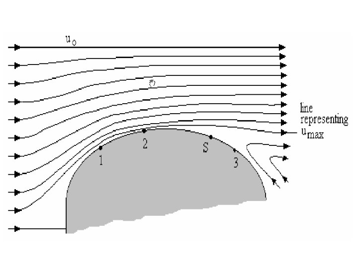
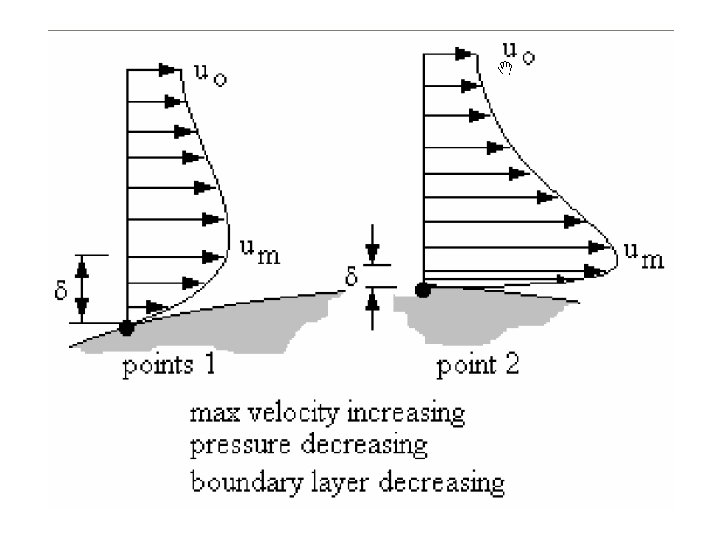
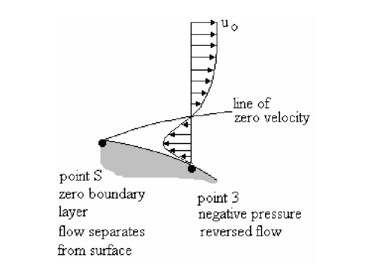
Pressure Gradients in Boundary-Layer Flow

Drag • Drag Coefficient with or

Drag • Pure Friction Drag: Flat Plate Parallel to the Flow • Pure Pressure Drag: Flat Plate Perpendicular to the Flow • Friction and Pressure Drag: Flow over a Sphere and Cylinder • Streamlining

Drag • Flow over a Flat Plate Parallel to the Flow: Friction Drag Boundary Layer can be 100% laminar, partly laminar and partly turbulent, or essentially 100% turbulent; hence several different drag coefficients are available

Drag • Flow over a Flat Plate Parallel to the Flow: Friction Drag (Continued) Laminar BL: Turbulent BL: … plus others for transitional flow

Drag Coefficient 0. 140 0. 120 0. 100 CD Laminar 0. 080 CD Turbulen 0. 060 0. 040 0. 020 0. 000 1 E+02 1 E+03 1 E+04 1 E+05 1 E+06 1 E+07 1 E+08 1 E+09

Drag • Flow over a Flat Plate Perpendicular to the Flow: Pressure Drag coefficients are usually obtained empirically

Drag • Flow over a Flat Plate Perpendicular to the Flow: Pressure Drag (Continued)

Drag • Flow over a Sphere and Cylinder: Friction and Pressure Drag

Drag • Flow over a Sphere and Cylinder: Friction and Pressure Drag (Continued)

Streamlining • Used to Reduce Wake and Pressure Drag

Lift • Mostly applies to Airfoils Note: Based on planform area Ap

Lift • Examples: NACA 23015; NACA 662 -215

Lift • Induced Drag

Lift • Induced Drag (Continued) Reduction in Effective Angle of Attack: Finite Wing Drag Coefficient:

Lift • Induced Drag (Continued)

The End Terima kasih Free Powerpoint Templates 73 Page 73