Kodak moments 3 D Visualization and Color CS

Kodak moments 3 -D Visualization and Color CS 112 Scientific Computation Department of Computer Science Wellesley College

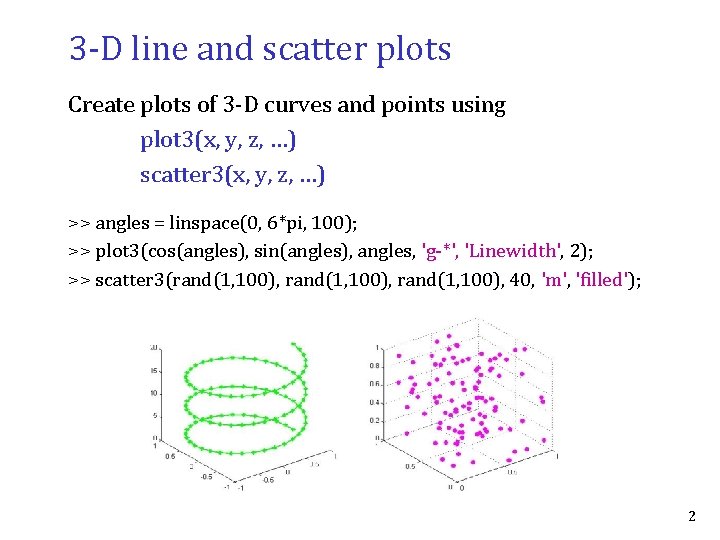
3 -D line and scatter plots Create plots of 3 -D curves and points using plot 3(x, y, z, …) scatter 3(x, y, z, …) >> angles = linspace(0, 6*pi, 100); >> plot 3(cos(angles), sin(angles), angles, 'g-*', 'Linewidth', 2); >> scatter 3(rand(1, 100), 40, 'm', 'filled'); 2

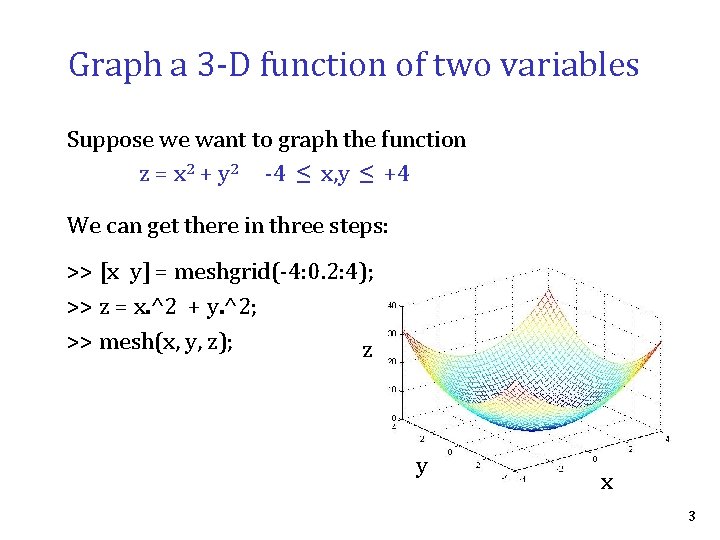
Graph a 3 -D function of two variables Suppose we want to graph the function z = x 2 + y 2 -4 ≤ x, y ≤ +4 We can get there in three steps: >> [x y] = meshgrid(-4: 0. 2: 4); >> z = x. ^2 + y. ^2; >> mesh(x, y, z); z y x 3

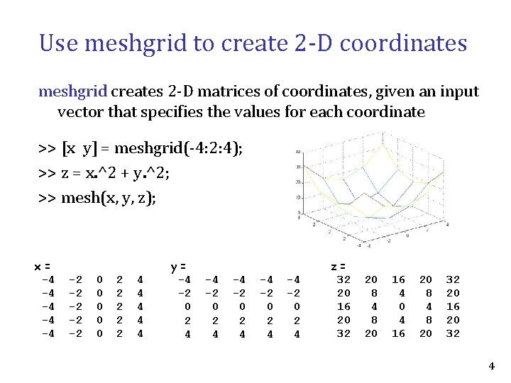
Use meshgrid to create 2 -D coordinates meshgrid creates 2 -D matrices of coordinates, given an input vector that specifies the values for each coordinate >> [x y] = meshgrid(-4: 2: 4); >> z = x. ^2 + y. ^2; >> mesh(x, y, z); x= -4 -2 0 2 4 -4 -2 0 2 4 y= -4 -4 -4 -2 -2 -2 0 0 0 2 2 2 4 4 4 z= 32 20 16 20 32 20 8 4 8 20 16 4 0 4 16 20 8 4 8 20 32 20 16 20 32 4

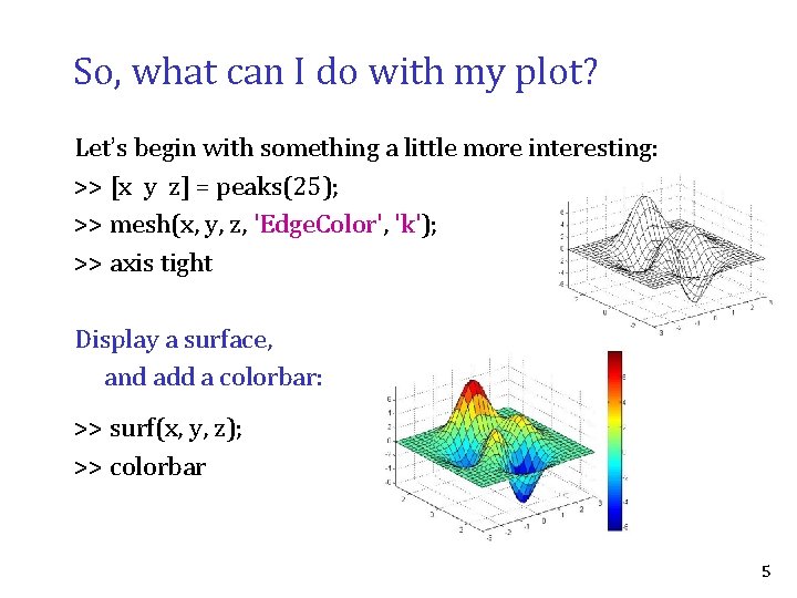
So, what can I do with my plot? Let’s begin with something a little more interesting: >> [x y z] = peaks(25); >> mesh(x, y, z, 'Edge. Color', 'k'); >> axis tight Display a surface, and add a colorbar: >> surf(x, y, z); >> colorbar 5

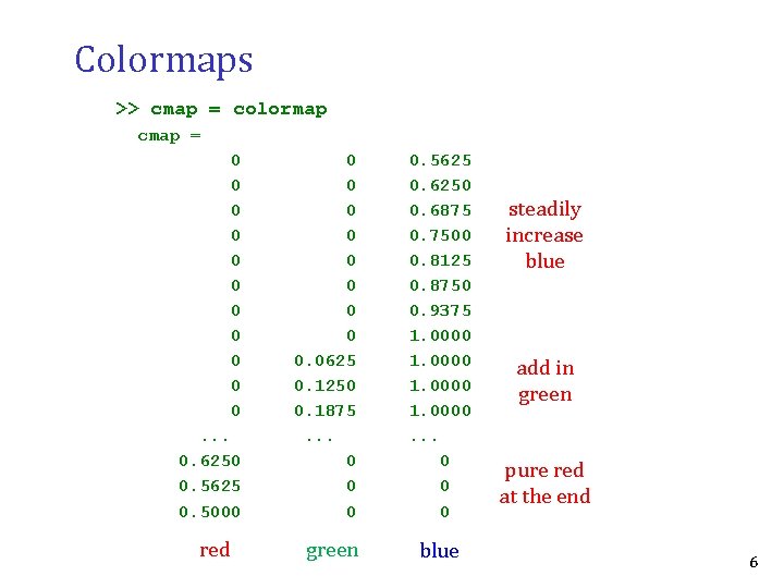
Colormaps >> cmap = colormap cmap = 0 0. 5625 0 0. 6250 0 0. 6875 0 0. 7500 0 0. 8125 0 0. 8750 0 0. 9375 0 1. 0000 0 0. 0625 1. 0000 0 0. 1250 1. 0000 0 0. 1875 1. 0000 . . . 0. 6250 0 0 0. 5625 0 0 0. 5000 0 0 red green blue steadily increase blue add in green pure red at the end 6

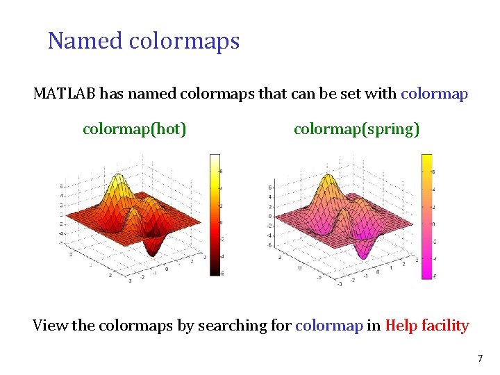
Named colormaps MATLAB has named colormaps that can be set with colormap(hot) colormap(spring) View the colormaps by searching for colormap in Help facility 7

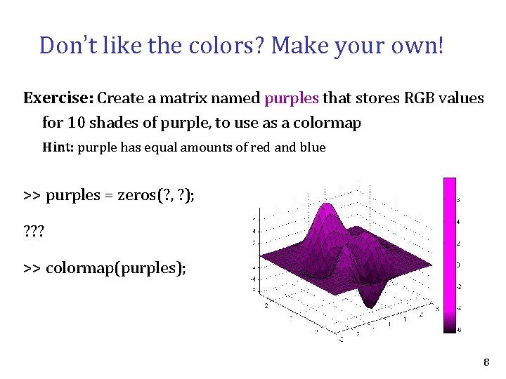
Don’t like the colors? Make your own! Exercise: Create a matrix named purples that stores RGB values for 10 shades of purple, to use as a colormap Hint: purple has equal amounts of red and blue >> purples = zeros(? , ? ); ? ? ? >> colormap(purples); 8

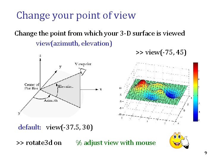
Change your point of view Change the point from which your 3 -D surface is viewed view(azimuth, elevation) >> view(-75, 45) default: view(-37. 5, 30) >> rotate 3 d on % adjust view with mouse 9

Add shading… Create a shaded surface using built-in shading methods >> [x y z] = sphere(20); >> surf(x, y, z); >> colormap(gray) >> shading faceted >> shading flat >> shading interp 10

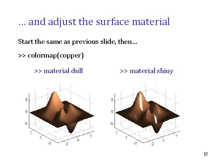
Add a light source… >> [x y z] = peaks(25); >> surf(x, y, z); >> axis tight >> colormap(gray) >> shading interp >> light('Position', [0 -1 0]) >> lighting phong 11

… and adjust the surface material Start the same as previous slide, then… >> colormap(copper) >> material dull >> material shiny 12

Contour plots >> [x y z] = peaks(25); >> contour(x, y, z, 20, 'Linewidth', 2) like a topographical map 13

Color images >> [x y z] = peaks(25); >> imagesc(z) >> colormap(gray) >> colormap(hot) 14