Knowing What to Do Knowing How to Do

Knowing What to Do Knowing How to Do It Getting Better Every Day Acceptance Sampling Webinar 20101129 1

Acceptance Sampling I Acceptance Sampling Webinar 20101129 2

What you will learn ¨ The purpose of Sampling ¨ How to draw a statistically valid Sample ¨ How to Develop a Sampling Plan ¨ How to construct an O-C curve for your sampling plan ¨ How to use (and understand) ANSI/ASQ Z 1. 4 ¨ How to use ANSI/ASQ Z 1. 9 ¨ Assessing Inspection Economics Acceptance Sampling Webinar 20101129 3

What is Sampling refers to the practice of evaluating (inspecting) a portion -the sample - of a lot – the population – for the purpose of inferring information about the lot. Statistically speaking, the properties of the sample distribution are used to infer the properties of the population (lot) distribution. An accept/reject decision is normally made based on the results of the sample Sampling is an Audit practice Acceptance Sampling Webinar 20101129 4

Why Sample? ¨ Economy Ø Less inspection labor Ø Less time ¨ Less handling damage ¨ Provides check on process control ¨ Fewer errors ? ? ? Ø i. e. inspection accuracy Acceptance Sampling Webinar 20101129 5

What does Sampling not do? ¨ Does not provide detailed information of lot quality ¨ Does not provide judgment of fitness for use (of rejected items) ¨ Does not guarantee elimination of defectives – any AQL permits defectives Acceptance Sampling Webinar 20101129 6

Sampling Caveats ¨ Size of sample is more important than percentage of lot ¨ Only random samples are statistically valid ¨ Access to samples does not guarantee randomness ¨ Acceptance sampling can place focus on wrong place Ø Supplier should provide evidence of quality Ø Focus should be on process control ¨ Misuse of sampling plans can be costly and misleading. ¨ No such thing as a single representative sample Acceptance Sampling Webinar 20101129 7

Representative Sample? There is no such thing as a single representative sample Why? ¨ Draw repeated samples of 5 from a normally distributed population. ¨ Record the X-bar (mean) and s (std. dev) for each sample ¨ What is the result? Acceptance Sampling Webinar 20101129 8

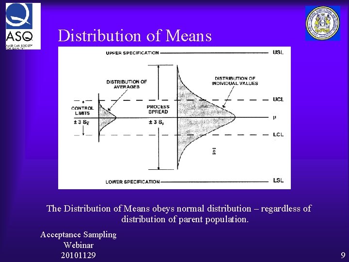
Distribution of Means The Distribution of Means obeys normal distribution – regardless of distribution of parent population. Acceptance Sampling Webinar 20101129 9

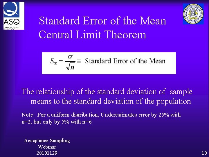
Standard Error of the Mean Central Limit Theorem The relationship of the standard deviation of sample means to the standard deviation of the population Note: For a uniform distribution, Underestimates error by 25% with n=2, but only by 5% with n=6 Acceptance Sampling Webinar 20101129 10

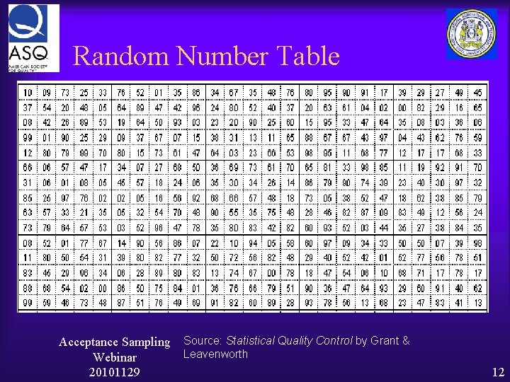
The Random Sample At any one time, each of the remaining items in the population has an equal chance of being the next item selected One method is to use a table of Random Numbers (handout from Grant & Leavenworth) Ø Enter the table Randomly ( like pin-the-tail-on-the-donkey) Ø Proceed in a predetermined direction – up, down, across Ø Discard numbers which cannot be applied to the sample Acceptance Sampling Webinar 20101129 11

Random Number Table Acceptance Sampling Webinar 20101129 Source: Statistical Quality Control by Grant & Leavenworth 12

Stratified Sampling ¨ Random samples are selected from a “homogeneous lot”. Often, the parts may not be homogeneous because they were produced on different machines, by different operators, in different plants, etc. ¨ With stratified sampling, random samples are drawn from each “group” of processes that are different from other groups. Acceptance Sampling Webinar 20101129 13

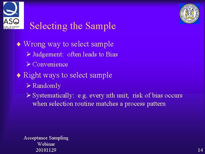
Selecting the Sample ¨ Wrong way to select sample Ø Judgement: often leads to Bias Ø Convenience ¨ Right ways to select sample Ø Randomly Ø Systematically: e. g. every nth unit; risk of bias occurs when selection routine matches a process pattern Acceptance Sampling Webinar 20101129 14

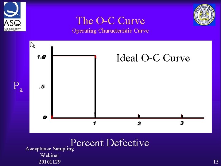
The O-C Curve Operating Characteristic Curve Ideal O-C Curve Pa Percent Defective Acceptance Sampling Webinar 20101129 15

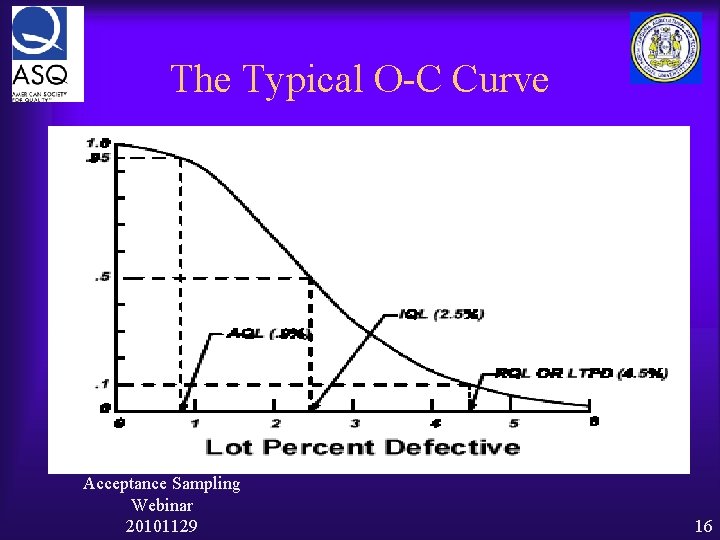
The Typical O-C Curve Acceptance Sampling Webinar 20101129 16

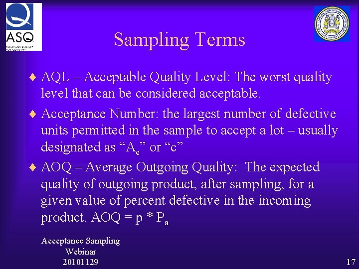
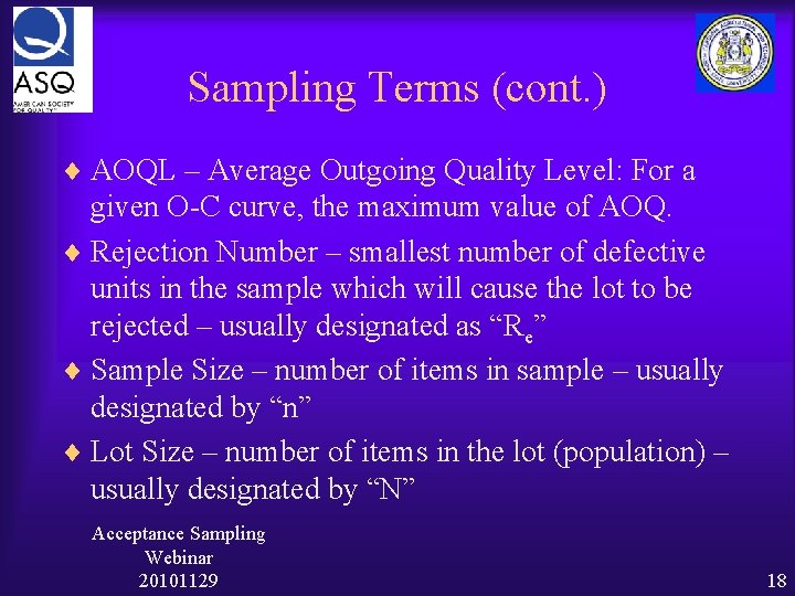
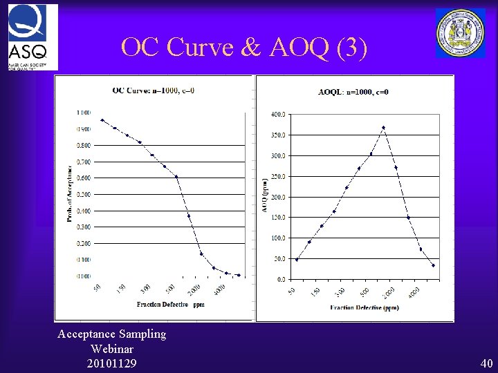
Sampling Terms ¨ AQL – Acceptable Quality Level: The worst quality level that can be considered acceptable. ¨ Acceptance Number: the largest number of defective units permitted in the sample to accept a lot – usually designated as “Ac” or “c” ¨ AOQ – Average Outgoing Quality: The expected quality of outgoing product, after sampling, for a given value of percent defective in the incoming product. AOQ = p * Pa Acceptance Sampling Webinar 20101129 17

Sampling Terms (cont. ) ¨ AOQL – Average Outgoing Quality Level: For a given O-C curve, the maximum value of AOQ. ¨ Rejection Number – smallest number of defective units in the sample which will cause the lot to be rejected – usually designated as “Re” ¨ Sample Size – number of items in sample – usually designated by “n” ¨ Lot Size – number of items in the lot (population) – usually designated by “N” Acceptance Sampling Webinar 20101129 18

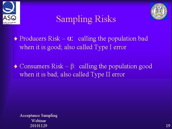
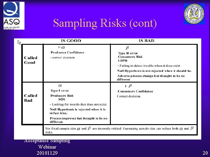
Sampling Risks ¨ Producers Risk – α: calling the population bad when it is good; also called Type I error ¨ Consumers Risk – β: calling the population good when it is bad; also called Type II error Acceptance Sampling Webinar 20101129 19

Sampling Risks (cont) Acceptance Sampling Webinar 20101129 20

Acceptance Sampling II Acceptance Sampling Webinar 20101129 21

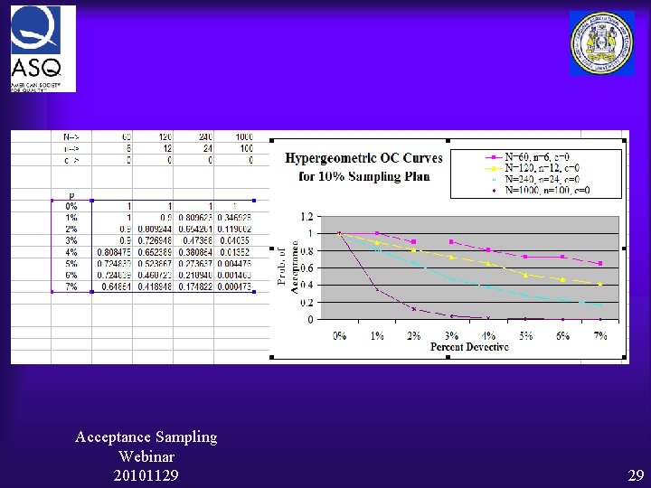
Constructing the O-C curve We will do the following O-C curves Ø Use Hyper-geometric and Poisson for each of the following • • N=60, n=6, Ac = 2 N=200, n=20, Ac = 2 N=1000, n=100, Ac = 2 N=1000, n=6, Ac = 2 Let’s do k (Ac, c - # of successes) = 0 first Acceptance Sampling Webinar 20101129 22

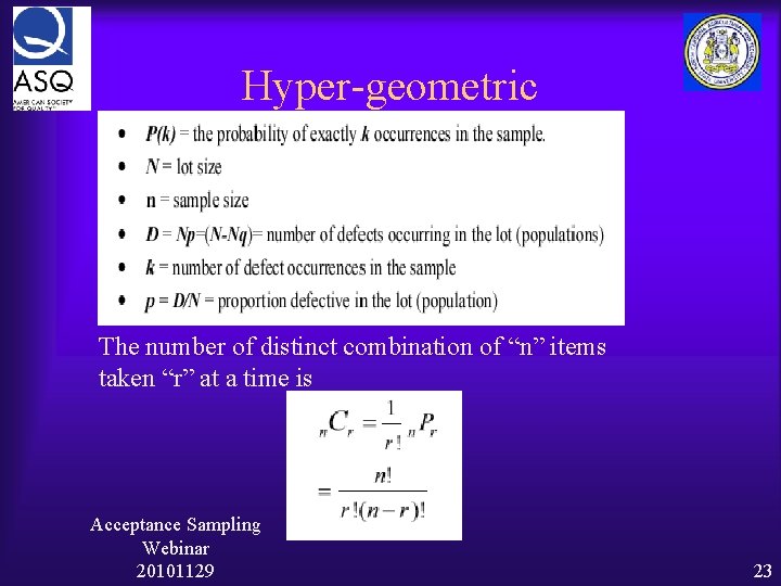
Hyper-geometric The number of distinct combination of “n” items taken “r” at a time is Acceptance Sampling Webinar 20101129 23

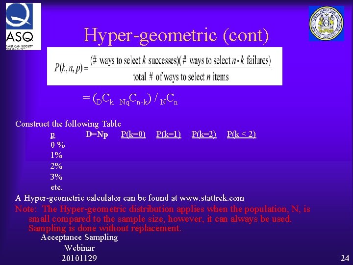
Hyper-geometric (cont) = ( DC k Nq. Cn-k) / NC n Construct the following Table p D=Np P(k=0) P(k=1) P(k=2) P(k ≤ 2) 0% 1% 2% 3% etc. A Hyper-geometric calculator can be found at www. stattrek. com Note: The Hyper-geometric distribution applies when the population, N, is small compared to the sample size, however, it can always be used. Sampling is done without replacement. Acceptance Sampling Webinar 20101129 24

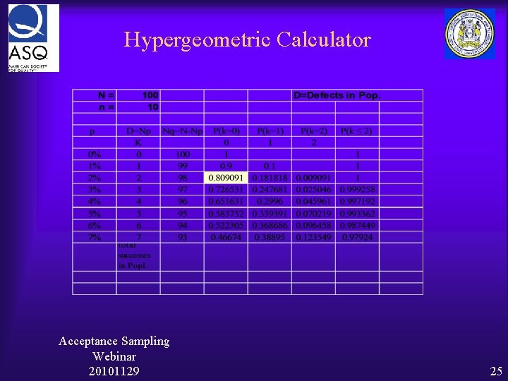
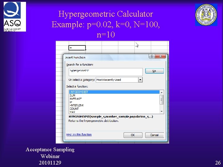
Hypergeometric Calculator Acceptance Sampling Webinar 20101129 25

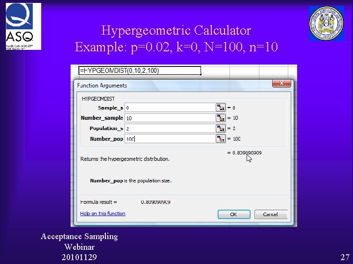
Hypergeometric Calculator Example: p=0. 02, k=0, N=100, n=10 Acceptance Sampling Webinar 20101129 26

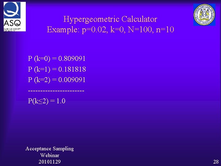
Hypergeometric Calculator Example: p=0. 02, k=0, N=100, n=10 Acceptance Sampling Webinar 20101129 27

Hypergeometric Calculator Example: p=0. 02, k=0, N=100, n=10 P (k=0) = 0. 809091 P (k=1) = 0. 181818 P (k=2) = 0. 009091 -----------P(k≤ 2) = 1. 0 Acceptance Sampling Webinar 20101129 28

Acceptance Sampling Webinar 20101129 29

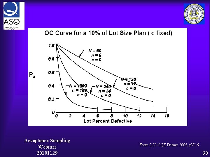
Acceptance Sampling Webinar 20101129 From QCI-CQE Primer 2005, p. VI-9 30

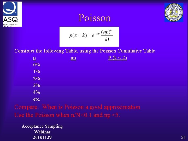
Poisson Construct the following Table, using the Poisson Cumulative Table p np P (k ≤ 2) 0% 1% 2% 3% 4% etc. Compare. When is Poisson a good approximation Use the Poisson when n/N˂0. 1 and np ˂5. Acceptance Sampling Webinar 20101129 31

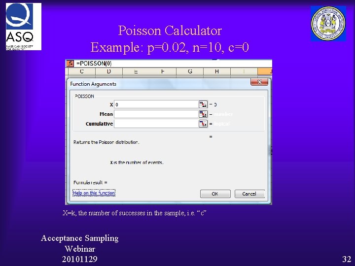
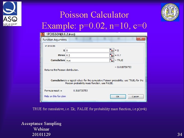
Poisson Calculator Example: p=0. 02, n=10, c=0 X=k, the number of successes in the sample, i. e. “c” Acceptance Sampling Webinar 20101129 32

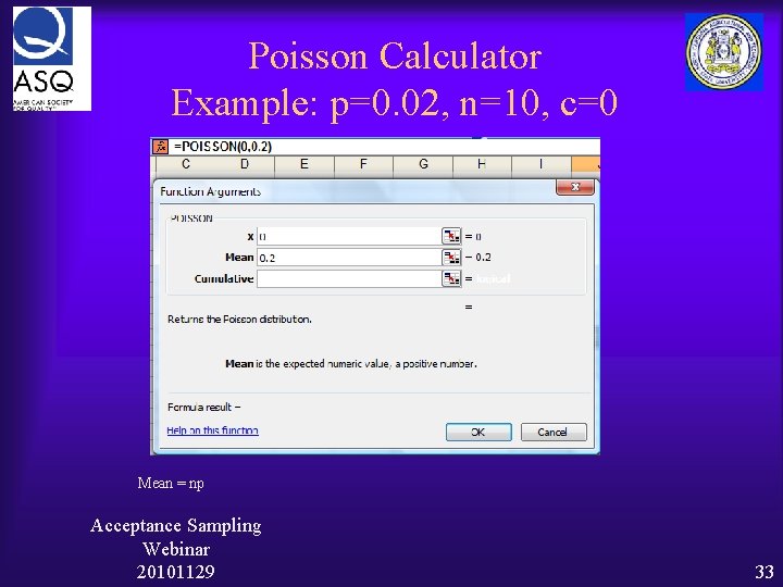
Poisson Calculator Example: p=0. 02, n=10, c=0 Mean = np Acceptance Sampling Webinar 20101129 33

Poisson Calculator Example: p=0. 02, n=10, c=0 TRUE for cumulative, i. e. Σk; FALSE for probability mass function, i. e. p(x=k) Acceptance Sampling Webinar 20101129 34

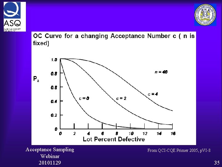
Acceptance Sampling Webinar 20101129 From QCI-CQE Primer 2005, p. VI-8 35

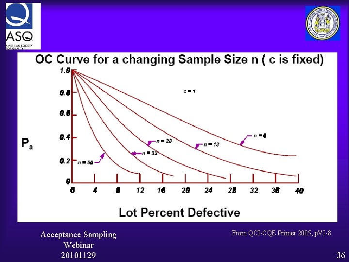
Acceptance Sampling Webinar 20101129 From QCI-CQE Primer 2005, p. VI-8 36

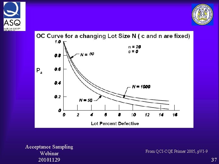
Acceptance Sampling Webinar 20101129 From QCI-CQE Primer 2005, p. VI-9 37

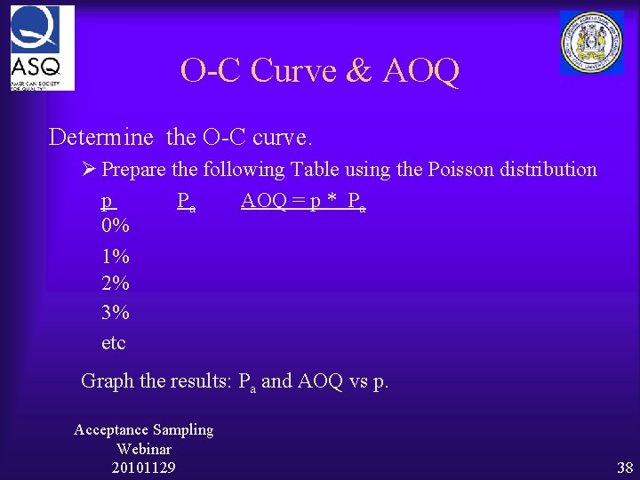
O-C Curve & AOQ Determine the O-C curve. Ø Prepare the following Table using the Poisson distribution p Pa AOQ = p * Pa 0% 1% 2% 3% etc Graph the results: Pa and AOQ vs p. Acceptance Sampling Webinar 20101129 38

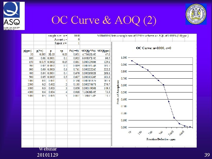
OC Curve & AOQ (2) Acceptance Sampling Webinar 20101129 39

OC Curve & AOQ (3) Acceptance Sampling Webinar 20101129 40

Acceptance Sampling III Acceptance Sampling Webinar 20101129 41

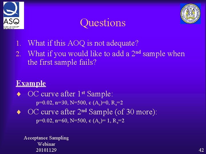
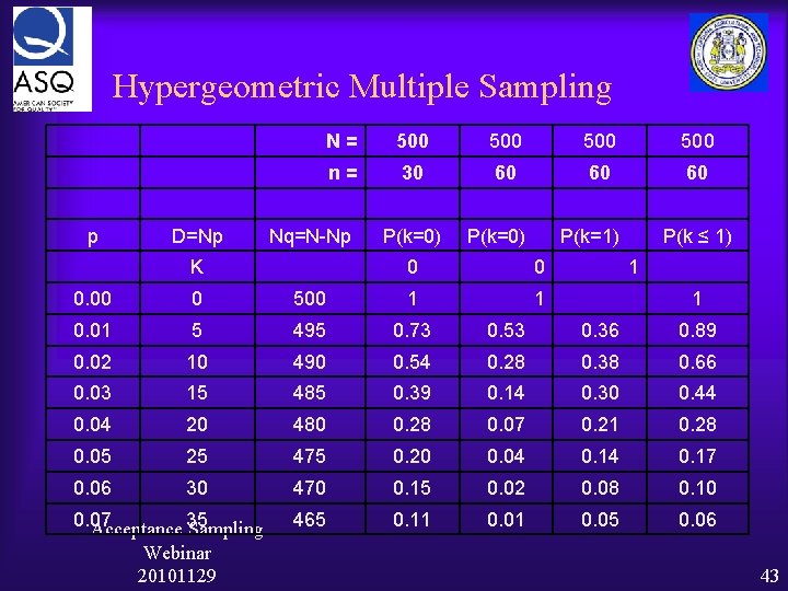
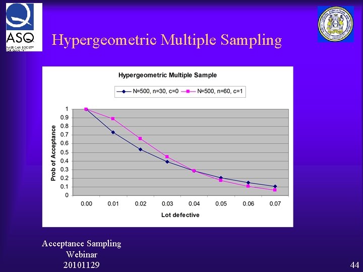
Questions 1. What if this AOQ is not adequate? 2. What if you would like to add a 2 nd sample when the first sample fails? Example ¨ OC curve after 1 st Sample: p=0. 02, n=30, N=500, c (Ac)=0, Re=2 ¨ OC curve after 2 nd Sample (of 30 more): p=0. 02, n=60, N=500, c (Ac)= 1, Re=2 Acceptance Sampling Webinar 20101129 42

Hypergeometric Multiple Sampling N= 500 500 n= 30 60 60 60 P(k=0) P(k=1) p D=Np Nq=N-Np P(k=0) K 0 0 0. 00 0 500 1 1 0. 01 5 495 0. 73 0. 53 0. 36 0. 89 0. 02 10 490 0. 54 0. 28 0. 38 0. 66 0. 03 15 485 0. 39 0. 14 0. 30 0. 44 0. 04 20 480 0. 28 0. 07 0. 21 0. 28 0. 05 25 475 0. 20 0. 04 0. 17 0. 06 30 470 0. 15 0. 02 0. 08 0. 10 465 0. 11 0. 05 0. 06 0. 07 Acceptance 35 Sampling Webinar 20101129 P(k ≤ 1) 1 1 43

Hypergeometric Multiple Sampling Acceptance Sampling Webinar 20101129 44

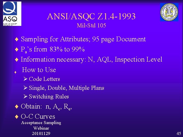
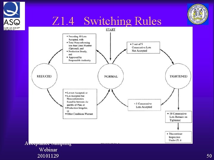
ANSI/ASQC Z 1. 4 -1993 Mil-Std 105 ¨ Sampling for Attributes; 95 page Document ¨ Pa’s from 83% to 99% ¨ Information necessary: N, AQL, Inspection Level ¨ How to Use Ø Code Letters Ø Single, Double, Multiple Plans Ø Switching Rules ¨ Obtain: n, Ac, Re, ¨ O-C Curves Acceptance Sampling Webinar 20101129 45

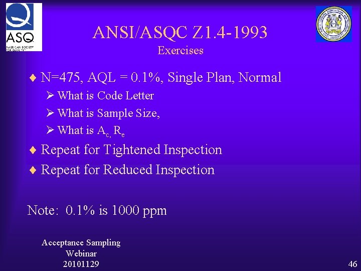
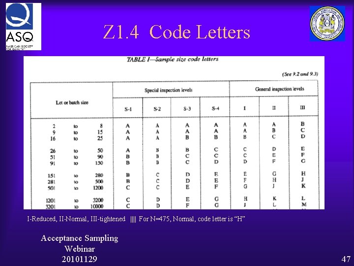
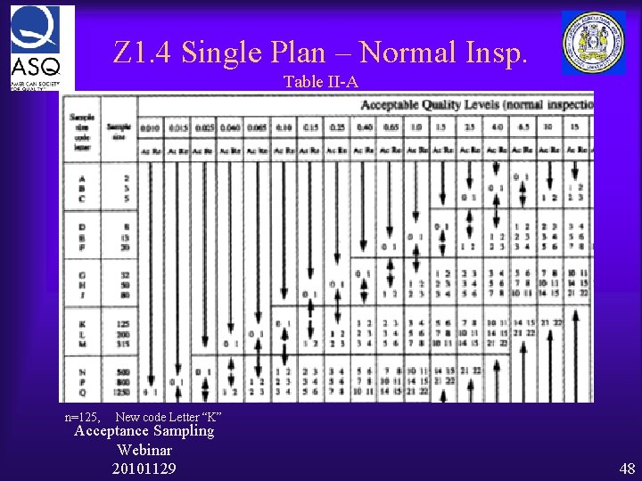
ANSI/ASQC Z 1. 4 -1993 Exercises ¨ N=475, AQL = 0. 1%, Single Plan, Normal Ø What is Code Letter Ø What is Sample Size, Ø What is Ac, Re ¨ Repeat for Tightened Inspection ¨ Repeat for Reduced Inspection Note: 0. 1% is 1000 ppm Acceptance Sampling Webinar 20101129 46

Z 1. 4 Code Letters I-Reduced, II-Normal, III-tightened |||| For N=475, Normal, code letter is “H” Acceptance Sampling Webinar 20101129 47

Z 1. 4 Single Plan – Normal Insp. Table II-A n=125, New code Letter “K” Acceptance Sampling Webinar 20101129 48

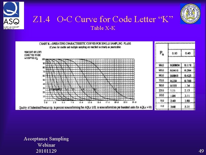
Z 1. 4 O-C Curve for Code Letter “K” Table X-K Acceptance Sampling Webinar 20101129 49

Z 1. 4 Switching Rules Acceptance Sampling Webinar 20101129 50

ANSI/ASQC Z 1. 4 -1993 What happens when AQL =. 1% isn’t good enough AQL = 0. 1% => 1000 ppm ¨ Is Z 1. 4 Adequate? ¨ How would you decide? ¨ If not, what would you do? ¨ Construct O-C curve for n=1000, c=0 (Poisson). Use 100 ppm < p < 5000 ppm (see slides 38 & 39) Acceptance Sampling Webinar 20101129 51

ANSI/ASQC Z 1. 9 -1993 Mil-Std 414 Sampling for Variables; 110 page Document Four Sections in the document ¨ Section A: General description of Plans ¨ Section B: Plans used when variability is unknown (Std. deviation method is used) ¨ Section C: Plans used when variability is unknown (range method is used) ¨ Section D: Plans used when the variability is known. Acceptance Sampling Webinar 20101129 52

ANSI/ASQC Z 1. 9 -1993 Mil-Std 414 ¨ Information necessary: N, AQL, Inspection Level ¨ How to Use Ø Code Letters Ø Single or Double Limit, Std. Dev or Range Method Plans Ø Switching Rules ¨ Obtain: Code Letter, n, Accept/Reject criteria, critical statistic (k) ¨ O-C Curves Acceptance Sampling Webinar 20101129 53

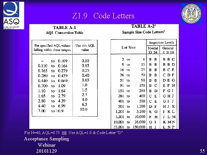
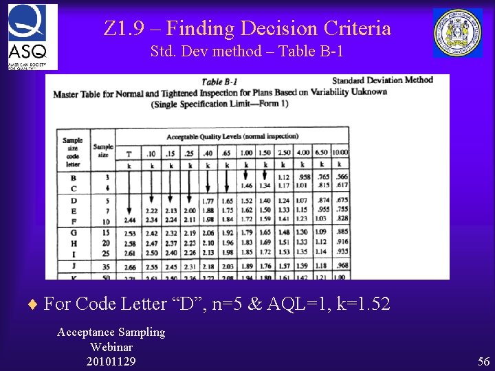
ANSI/ASQC Z 1. 9 -1993 Exercise (From QCI, CQE Primer, p. VI-37) The specified max. temp for operation of a device is 209 F. A lot of 40 is submitted for inspection. Use Normal (Level II) with AQL = 0. 75%. The Std. Dev. is unknown. Use Std. Dev. Method, variation unknown Ø Find Code Letter, Sample Size, k Ø Should lot be accepted or rejected Acceptance Sampling Webinar 20101129 54

Z 1. 9 Code Letters For N=40, AQL=0. 75 |||||| Use AQL=1. 0 & Code Letter “D” Acceptance Sampling Webinar 20101129 55

Z 1. 9 – Finding Decision Criteria Std. Dev method – Table B-1 ¨ For Code Letter “D”, n=5 & AQL=1, k=1. 52 Acceptance Sampling Webinar 20101129 56

ANSI/ASQC Z 1. 9 -1993 What is “k” is a critical statistic (term used in hypothesis testing). It defines the maximum area of the distribution which can be above the USL. When Qcalc > k, there is less of distribution above Qcalc than above “k” and lot is accepted. (Compare to “Z” table) Increasing (USL - X-bar) increases Pa Acceptance Sampling Webinar 20101129 57

ANSI/ASQC Z 1. 9 -1993 Exercise Solution The five reading are 197 F, 188 F, 184 F, 205 F, 201 F. ¨ X-bar (mean) = 195 F ¨ S (Std. Dev) = 8. 8 F ¨ Qcalc = (USL – X-bar)/s = 1. 59 ¨ Because Qcalc = 1. 59 is greater than k=1. 52, lot is accepted Acceptance Sampling Webinar 20101129 58

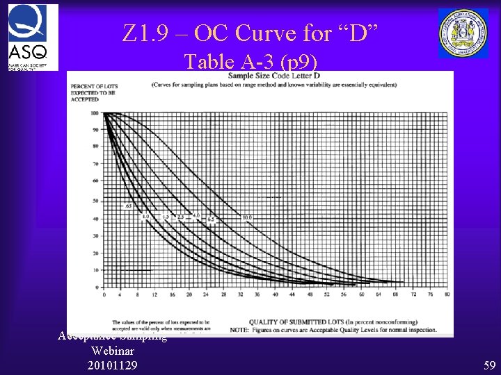
Z 1. 9 – OC Curve for “D” Table A-3 (p 9) Acceptance Sampling Webinar 20101129 59

ANSI/ASQC Z 1. 9 -1993 Another Exercise ¨ Same information as before ¨ AQL = 0. 1 ¨ Find Code Letter, n, k ¨ Accept or Reject Lot? Acceptance Sampling Webinar 20101129 60

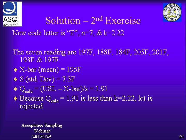
Solution – 2 nd Exercise New code letter is “E”, n=7, & k=2. 22 The seven reading are 197 F, 188 F, 184 F, 205 F, 201 F, 193 F & 197 F. ¨ X-bar (mean) = 195 F ¨ S (std. Dev) = 7. 3 F ¨ Qcalc = (USL – X-bar)/s = 1. 91 ¨ Because Qcalc = 1. 91 is less than k=2. 22, lot is rejected Acceptance Sampling Webinar 20101129 61

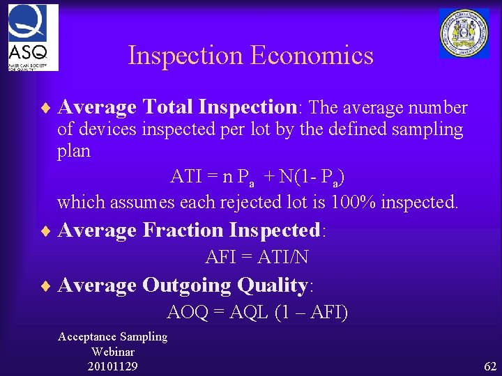
Inspection Economics ¨ Average Total Inspection: The average number of devices inspected per lot by the defined sampling plan ATI = n Pa + N(1 - Pa) which assumes each rejected lot is 100% inspected. ¨ Average Fraction Inspected: AFI = ATI/N ¨ Average Outgoing Quality: AOQ = AQL (1 – AFI) Acceptance Sampling Webinar 20101129 62

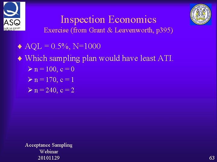
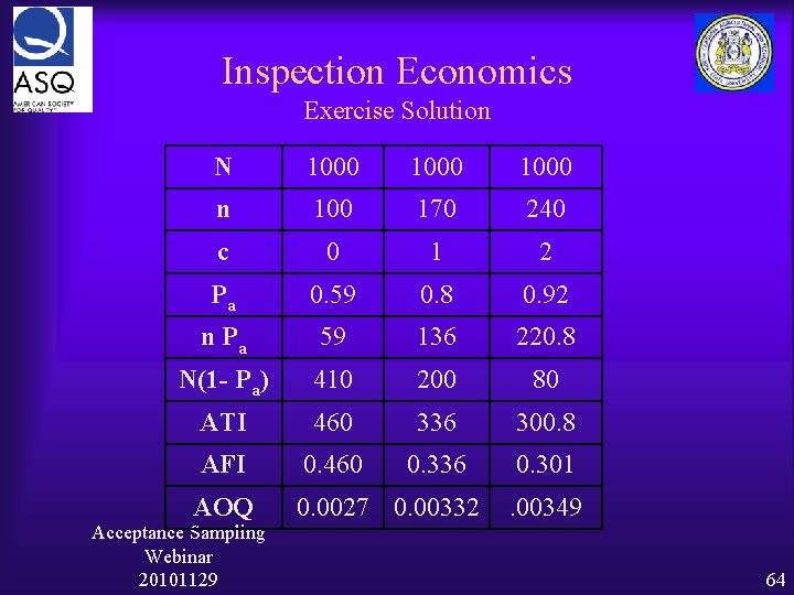
Inspection Economics Exercise (from Grant & Leavenworth, p 395) ¨ AQL = 0. 5%, N=1000 ¨ Which sampling plan would have least ATI. Ø n = 100, c = 0 Ø n = 170, c = 1 Ø n = 240, c = 2 Acceptance Sampling Webinar 20101129 63

Inspection Economics Exercise Solution N 1000 n 100 170 240 c 0 1 2 Pa 0. 59 0. 8 0. 92 n Pa 59 136 220. 8 N(1 - Pa) 410 200 80 ATI 460 336 300. 8 AFI 0. 460 0. 336 0. 301 AOQ 0. 0027 0. 00332 Acceptance Sampling Webinar 20101129 . 00349 64

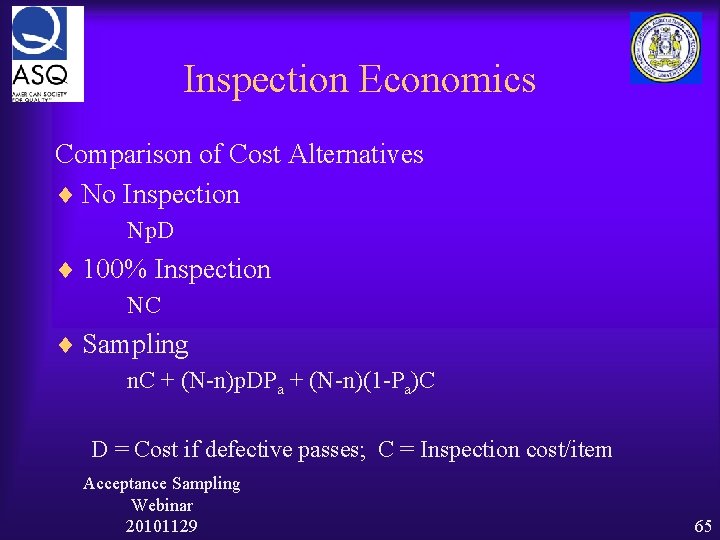
Inspection Economics Comparison of Cost Alternatives ¨ No Inspection Np. D ¨ 100% Inspection NC ¨ Sampling n. C + (N-n)p. DPa + (N-n)(1 -Pa)C D = Cost if defective passes; C = Inspection cost/item Acceptance Sampling Webinar 20101129 65

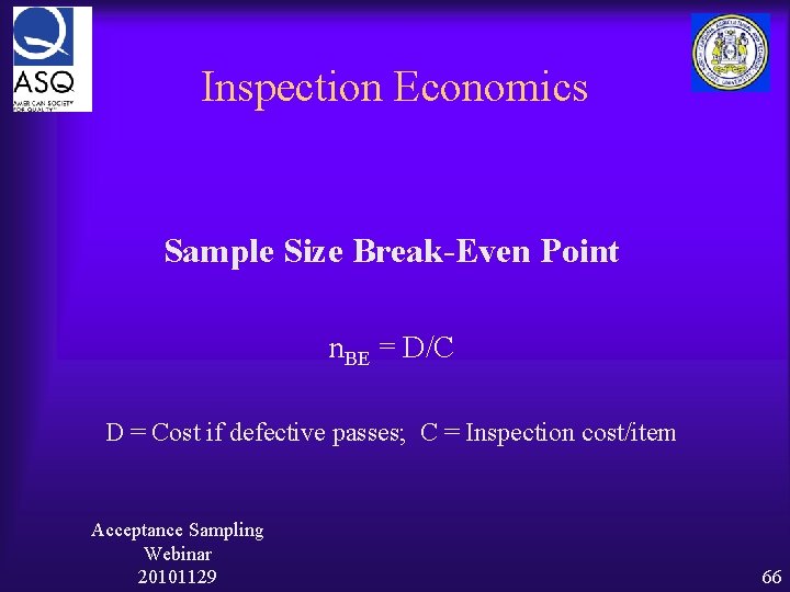
Inspection Economics Sample Size Break-Even Point n. BE = D/C D = Cost if defective passes; C = Inspection cost/item Acceptance Sampling Webinar 20101129 66

Resources ¨ American Society for Quality Ø Quality Press Ø www. asq. org ¨ ASQ/NC A&T partnership quality courses Ø CQIA, CMI, CQT, CQA, CQMgr, CQE, CSSBB Ø Quality Progress Magazine Ø And others ¨ Web-Sites Ø www. stattrek. com – excellent basic stat site Ø http: //mathworld. wolfram. com/ - greaqt math and stat site Acceptance Sampling Webinar 20101129 67