King Fahd University of Petroleum Minerals Computer Engineering

![Little’s Formula • Little’s formula: E[N] = λE[T] i. e. For systems reaching steady Little’s Formula • Little’s formula: E[N] = λE[T] i. e. For systems reaching steady](https://slidetodoc.com/presentation_image_h/c513bbcaf61550d78772953cacd7eabd/image-9.jpg)

![M/M/1/K – Mean Number of Customers • Mean number of customers, E[N] is given M/M/1/K – Mean Number of Customers • Mean number of customers, E[N] is given](https://slidetodoc.com/presentation_image_h/c513bbcaf61550d78772953cacd7eabd/image-31.jpg)
![M/M/1/K – Mean Delay • The mean total delay E[T] is given by E[T] M/M/1/K – Mean Delay • The mean total delay E[T] is given by E[T]](https://slidetodoc.com/presentation_image_h/c513bbcaf61550d78772953cacd7eabd/image-34.jpg)
![Mean Waiting Time in M/G/1 – cont’d • Substituting back, yields λE[ 2] E[W] Mean Waiting Time in M/G/1 – cont’d • Substituting back, yields λE[ 2] E[W]](https://slidetodoc.com/presentation_image_h/c513bbcaf61550d78772953cacd7eabd/image-52.jpg)
![Mean Delay in M/G/1 – cont’d • The mean waiting time, E[T] is found Mean Delay in M/G/1 – cont’d • The mean waiting time, E[T] is found](https://slidetodoc.com/presentation_image_h/c513bbcaf61550d78772953cacd7eabd/image-53.jpg)
![Example 7: • Problem: Compare E[W] for M/M/1 and M/D/1 systems. • Answer: M/M/1: Example 7: • Problem: Compare E[W] for M/M/1 and M/D/1 systems. • Answer: M/M/1:](https://slidetodoc.com/presentation_image_h/c513bbcaf61550d78772953cacd7eabd/image-54.jpg)
![Example 8: cont’d • Solution: a) Average packet size, E[L] = 0. 3 512 Example 8: cont’d • Solution: a) Average packet size, E[L] = 0. 3 512](https://slidetodoc.com/presentation_image_h/c513bbcaf61550d78772953cacd7eabd/image-57.jpg)
- Slides: 57

King Fahd University of Petroleum & Minerals Computer Engineering Dept COE 540 – Computer Networks Term 082 Courtesy of: Dr. Ashraf S. Hasan Mahmoud 1

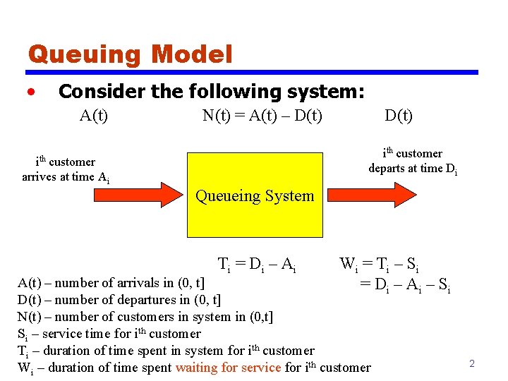
Queuing Model • Consider the following system: A(t) N(t) = A(t) – D(t) ith customer departs at time Di ith customer arrives at time Ai Queueing System T i = Di – Ai W i = T i – Si = Di – Ai – Si A(t) – number of arrivals in (0, t] D(t) – number of departures in (0, t] N(t) – number of customers in system in (0, t] Si – service time for ith customer Ti – duration of time spent in system for ith customer Wi – duration of time spent waiting for service for ith customer 2

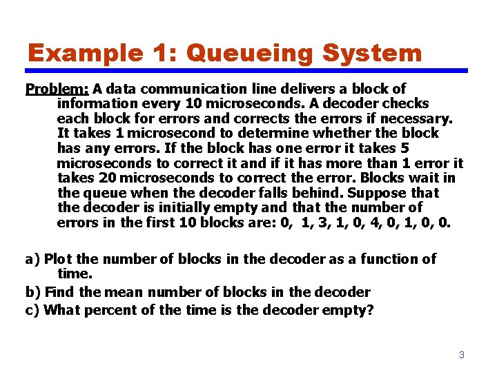
Example 1: Queueing System Problem: A data communication line delivers a block of information every 10 microseconds. A decoder checks each block for errors and corrects the errors if necessary. It takes 1 microsecond to determine whether the block has any errors. If the block has one error it takes 5 microseconds to correct it and if it has more than 1 error it takes 20 microseconds to correct the error. Blocks wait in the queue when the decoder falls behind. Suppose that the decoder is initially empty and that the number of errors in the first 10 blocks are: 0, 1, 3, 1, 0, 4, 0, 1, 0, 0. a) Plot the number of blocks in the decoder as a function of time. b) Find the mean number of blocks in the decoder c) What percent of the time is the decoder empty? 3

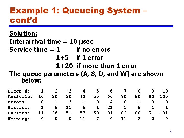
Example 1: Queueing System – cont’d Solution: Interarrival time = 10 μsec Service time = 1 if no errors 1+5 if 1 error 1+20 if more than 1 error The queue parameters (A, S, D, and W) are shown below: Block #: Arrivals: Errors: Service: Departs: Waiting: 1 10 0 1 11 0 2 20 1 6 26 0 3 30 3 21 51 0 4 40 1 6 57 11 5 50 0 1 58 7 6 60 4 21 81 0 7 70 0 1 82 11 8 80 1 6 88 2 9 90 0 1 91 0 10 100 0 1 101 0 4

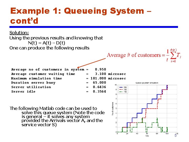
Example 1: Queueing System – cont’d Solution: Using the previous results and knowing that N(t) = A(t) – D(t) One can produce the following results Average no of customers in system Average customer waiting time Maximum simulation time Duration server busy Server utilization Server idle = 0. 950 = 3. 100 microsec = 101. 000 microsec = 65. 000 microsec = 0. 6436 = 0. 3564 The following Matlab code can be used to solve this queue system (Note the code is general – it solves any system provided the Arrivals vector A, and the service vector S) 5

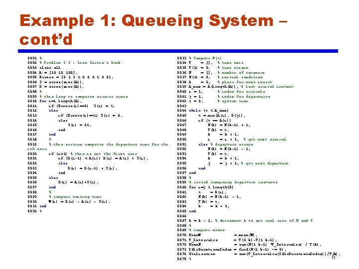
Example 1: Queueing System – cont’d 0001 % 0002 % Problem 9. 3 - Leon Garcia's book 0003 clear all 0004 A = [10: 100]; 0005 Errors = [0 1 3 1 0 4 0 1 0 0]; 0006 S = zeros(size(A)); 0007 D = zeros(size(A)); 0008 % 0009 % this loop to computes service times 0010 for i=1: length(A); 0011 if (Errors(i)==0) S(i) = 1; 0012 else 0013 if (Errors(i)==1) S(i) = 6; 0014 else 0015 S(i) = 21; 0016 end 0017 end 0018 % 0019 % this section computes the departure time for the ith user 0020 if (i>1) % this is not the first user 0021 if (D(i-1) < A(i)) D(i) = A(i) + S(i); 0022 else 0023 D(i) = D(i-1) + S(i); 0024 end 0025 else 0026 D(i) = A(i)+S(i); 0027 end 0028 % 0029 % compute waiting time 0030 W(i) = D(i) - A(i) - S(i); 0031 end 0032 % 0033 0034 0035 0036 0037 0038 0039 0040 0041 0042 0043 0044 0045 0046 0047 0048 0049 0050 0051 0052 0053 0054 0055 0056 0057 0058 0059 0060 0061 0062 0063 0064 0065 0066 0067 0068 0069 0070 0071 0072 0073 0074 0075 % Compute N(t) T = []; % time axis T(1) = 0; % time origin N = []; % number of cutomers N(1) = 0; % initial condition k = 2; % place for next insert A_max = A(length(A)); % last arrival instant i = 1; % index for arrivals j = 1; % index for departures t = 0; % system time while (t < A_max) t = min(A(i), D(j)); if (t == A(i)) N(k) = N(k-1) + 1; T(k) = t; k = k + 1; i = i + 1; % get next arrival else % departure occurs N(k) = N(k-1) - 1; T(k) = t; k = k + 1; j = j + 1; % get next departure end % % record remaining departure instants for i=j: 1: length(D) t = D(i); N(k) = N(k-1) - 1; T(k) = t; k = k + 1; end k = k - 1; % decrement k to get real size of N and T % % compute means Mean. W = mean(W); T_Intervales = T(2: k)-T(1: k-1); Mean. N = sum(N(1: k-1). *T_Intervales) / T(k); Idle. Durations. Index = find(N(1: k-1) ~= 0); Utilization = sum(T_Intervales(Idle. Durations. Index))/T(k); % 6

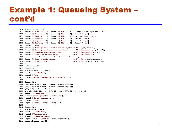
Example 1: Queueing System – cont’d 0076 0077 0078 0079 0080 0081 0082 0083 0084 0085 0086 0087 0088 0089 0090 0091 0092 0093 0094 0095 0096 0097 0098 0099 0100 0101 0102 0103 0104 0105 0106 0107 0108 0109 0110 0111 0112 0113 0114 0115 0116 % Display results fprintf('Block #: '); fprintf('%3 d ', [1: 1: length(A)]); fprintf('n'); fprintf('Arrivals: '); fprintf('%3 d ', A); fprintf('n'); fprintf('Errors: '); fprintf('%3 d ', Errors); fprintf('n'); fprintf('Service: '); fprintf('%3 d ', S); fprintf('n'); fprintf('Departs: '); fprintf('%3 d ', D); fprintf('n'); fprintf('Waiting: '); fprintf('%3 d ', W); fprintf('n'); fprintf('nn'); fprintf('Average no of customers in system = %7. 3 fn', Mean. N); fprintf('Average customer waiting time = %7. 3 f microsecn', Mean. W); fprintf('Maximum simulation time = %7. 3 f microsecn', T(k)); fprintf('Duration server busy = %7. 3 f microsecn', . . . sum(T_Intervales(Idle. Durations. Index))); fprintf('Server utilization = %7. 4 fn', Utilization); fprintf('Server idle = %7. 4 fn', 1. 0 -Utilization); % % Plot results figure(1) h = stairs(T, N); grid set(h, 'Line. Width', 3); xlabel('Time'); ylabel('No of customers in system, N(t)'); figure(2); [AT, AA] = stairs(A, cumsum(ones(size(A)))); [DT, DD] = stairs(D, cumsum(ones(size(D)))); [NT, NN] = stairs(T, N); h = plot(AT, AA, '-', DT, DD, '--r', NT, NN, '-. '); grid set(h, 'Line. Width', 3); title('Queue sysystem simulation'); ylabel('No of customers'); xlabel('Time'); legend('A(t)', 'D(t)', 'N(t)', 0); figure(3); h = stem(W); grid set(h, 'Line. Width', 3); ylabel('Waiting time'); xlabel('Customer index'); Legend. Str = ['Mean. W = ' num 2 str(Mean. W)]; legend(Legend. Str, 0); 7

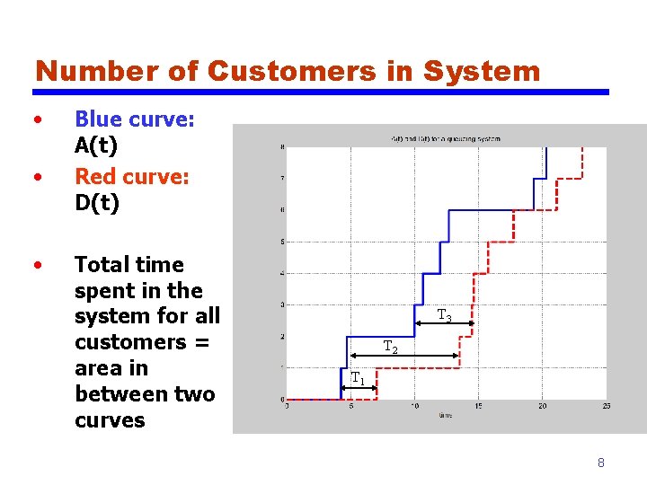
Number of Customers in System • • • Blue curve: A(t) Red curve: D(t) Total time spent in the system for all customers = area in between two curves T 3 T 2 T 1 8
![Littles Formula Littles formula EN λET i e For systems reaching steady Little’s Formula • Little’s formula: E[N] = λE[T] i. e. For systems reaching steady](https://slidetodoc.com/presentation_image_h/c513bbcaf61550d78772953cacd7eabd/image-9.jpg)
Little’s Formula • Little’s formula: E[N] = λE[T] i. e. For systems reaching steady state, the average number of customers in the system = average arrival rate average time spent in the system Holds for many service disciplines and for systems with arbitrary number of servers. It holds for many interpretations of the “system” as well. 9

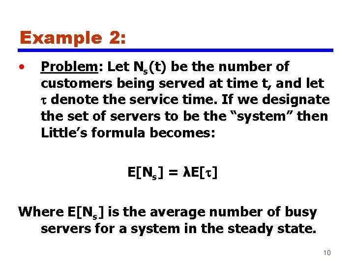
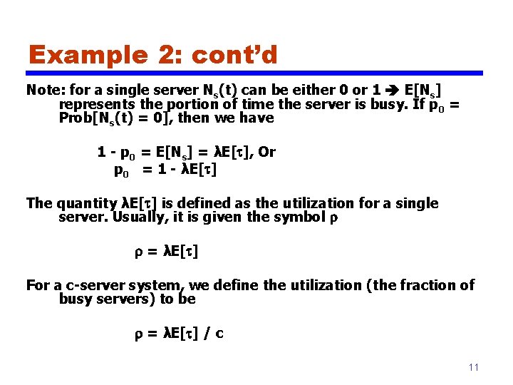
Example 2: • Problem: Let Ns(t) be the number of customers being served at time t, and let denote the service time. If we designate the set of servers to be the “system” then Little’s formula becomes: E[Ns] = λE[ ] Where E[Ns] is the average number of busy servers for a system in the steady state. 10

Example 2: cont’d Note: for a single server Ns(t) can be either 0 or 1 E[Ns] represents the portion of time the server is busy. If p 0 = Prob[Ns(t) = 0], then we have 1 - p 0 = E[Ns] = λE[ ], Or p 0 = 1 - λE[ ] The quantity λE[ ] is defined as the utilization for a single server. Usually, it is given the symbol = λE[ ] For a c-server system, we define the utilization (the fraction of busy servers) to be = λE[ ] / c 11

Example 3: Applications on Little’s Formula Refer to the slides for Dr. Waheed. The slides have 8 good examples! 12

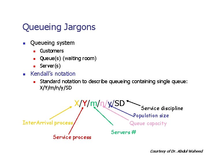
Queueing Jargons n Queueing system n n Customers Queue(s) (waiting room) Server(s) Kendall’s notation n Standard notation to describe queueing containing single queue: X/Y/m/n/y/SD Inter. Arrival process Service discipline Population size Queue capacity Servers # Courtesy of Dr. Abdul Waheed

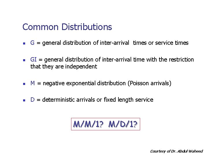
Common Distributions n n G = general distribution of inter-arrival times or service times GI = general distribution of inter-arrival time with the restriction that they are independent n M = negative exponential distribution (Poisson arrivals) n D = deterministic arrivals or fixed length service M/M/1? M/D/1? Courtesy of Dr. Abdul Waheed

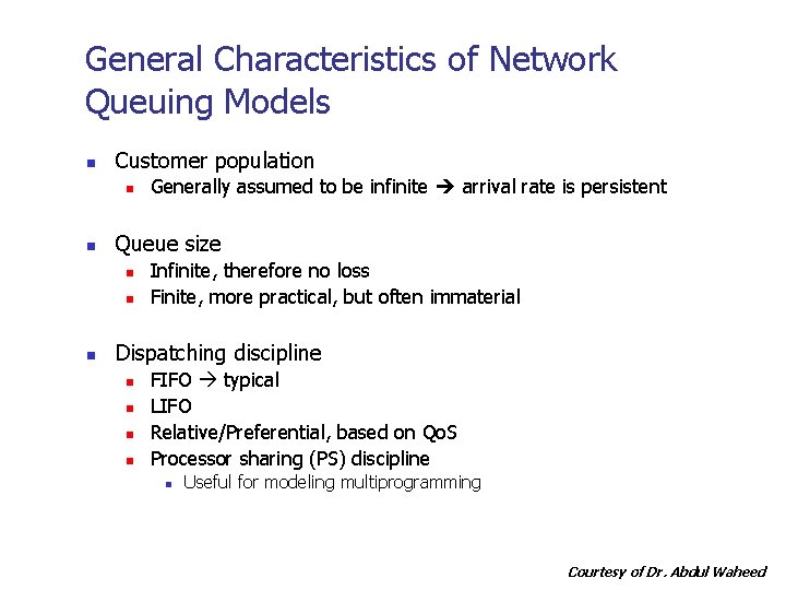
General Characteristics of Network Queuing Models n Customer population n n Queue size n n n Generally assumed to be infinite arrival rate is persistent Infinite, therefore no loss Finite, more practical, but often immaterial Dispatching discipline n n FIFO typical LIFO Relative/Preferential, based on Qo. S Processor sharing (PS) discipline n Useful for modeling multiprogramming Courtesy of Dr. Abdul Waheed

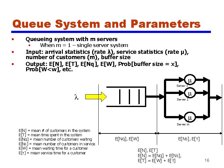
Queue System and Parameters • Queueing system with m servers • Input: arrival statistics (rate λ), service statistics (rate μ), number of customers (m), buffer size Output: E[N], E[T], E[Nq], E[W], Prob[buffer size = x], Prob[W<w], etc. • • When m = 1 – single server system μ Server 1 μ λ Server 2 μ Server m E[N] = mean # of customers in the system E[T] = mean time spent in the system E[Nq] = mean number of customers waiting E[Ns] = mean number of customers in service E[W] = mean waiting time for a customer E[τ] = mean service time for a customer E[Nq], E[W] E[Ns], E[τ] E[N], E[T] E[N] = E[Nq] + E[Ns], E[T] = E[W] + E[τ] 16

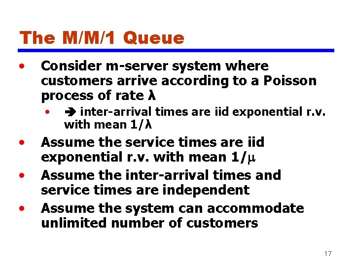
The M/M/1 Queue • Consider m-server system where customers arrive according to a Poisson process of rate λ • • inter-arrival times are iid exponential r. v. with mean 1/λ Assume the service times are iid exponential r. v. with mean 1/m Assume the inter-arrival times and service times are independent Assume the system can accommodate unlimited number of customers 17

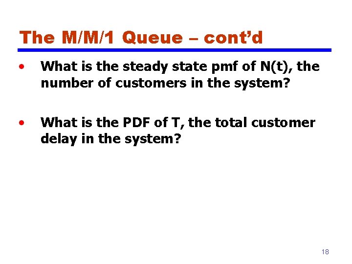
The M/M/1 Queue – cont’d • What is the steady state pmf of N(t), the number of customers in the system? • What is the PDF of T, the total customer delay in the system? 18

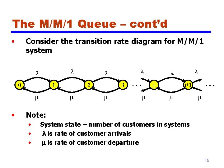
The M/M/1 Queue – cont’d • Consider the transition rate diagram for M/M/1 system l l 0 1 m • 2 m l l 3 m j m l l j+1 m m Note: • • • System state – number of customers in systems λ is rate of customer arrivals m is rate of customer departure 19

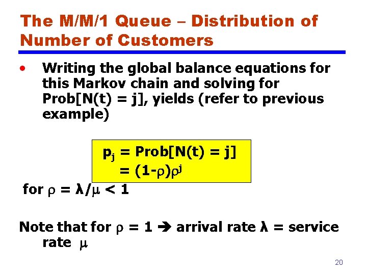
The M/M/1 Queue – Distribution of Number of Customers • Writing the global balance equations for this Markov chain and solving for Prob[N(t) = j], yields (refer to previous example) pj = Prob[N(t) = j] = (1 - ) j for = λ/m < 1 Note that for = 1 arrival rate λ = service rate m 20

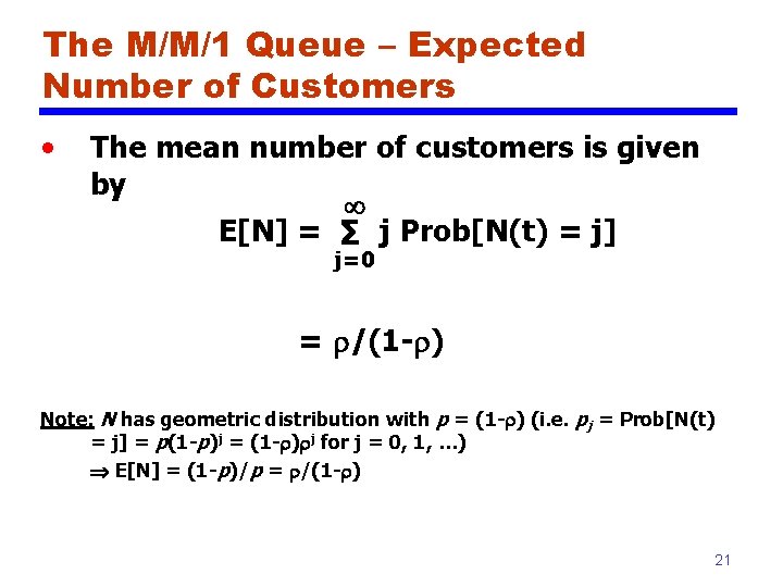
The M/M/1 Queue – Expected Number of Customers • The mean number of customers is given by E[N] = ∑ j Prob[N(t) = j] j=0 = /(1 - ) Note: N has geometric distribution with p = (1 - ) (i. e. pj = Prob[N(t) = j] = p(1 -p)j = (1 - ) j for j = 0, 1, …) E[N] = (1 -p)/p = /(1 - ) 21

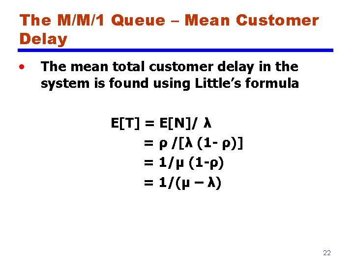
The M/M/1 Queue – Mean Customer Delay • The mean total customer delay in the system is found using Little’s formula E[T] = E[N]/ λ = ρ /[λ (1 - ρ)] = 1/μ (1 -ρ) = 1/(μ – λ) 22

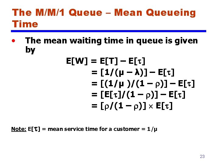
The M/M/1 Queue – Mean Queueing Time • The mean waiting time in queue is given by E[W] = E[T] – E[ ] = [1/(μ – λ)] – E[ ] = [(1/μ )/(1 – )] – E[ ] = [E[ ]/(1 – )] – E[ ] = [ /(1 – )] E[ ] Note: E[ ] = mean service time for a customer = 1/μ 23

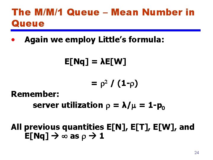
The M/M/1 Queue – Mean Number in Queue • Again we employ Little’s formula: E[Nq] = λE[W] = 2 / (1 - ) Remember: server utilization = λ/m = 1 -p 0 All previous quantities E[N], E[T], E[W], and E[Nq] as 1 24

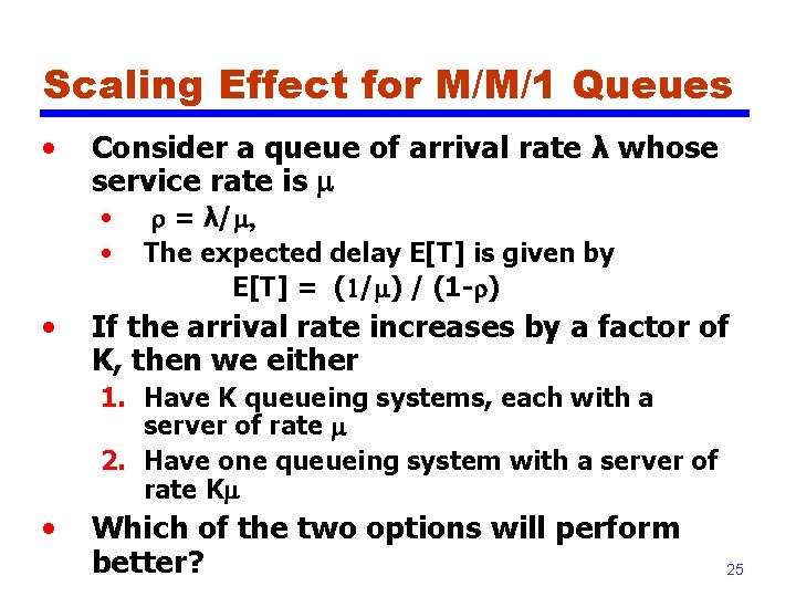
Scaling Effect for M/M/1 Queues • Consider a queue of arrival rate λ whose service rate is m • • • = λ/m, The expected delay E[T] is given by E[T] = (1/m) / (1 - ) If the arrival rate increases by a factor of K, then we either 1. Have K queueing systems, each with a server of rate m 2. Have one queueing system with a server of rate Km • Which of the two options will perform better? 25

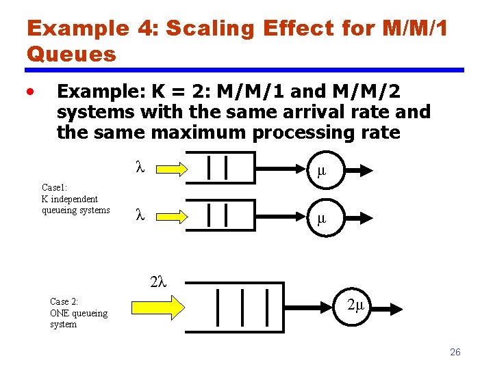
Example 4: Scaling Effect for M/M/1 Queues • Example: K = 2: M/M/1 and M/M/2 systems with the same arrival rate and the same maximum processing rate Case 1: K independent queueing systems λ μ 2λ Case 2: ONE queueing system 2μ 26

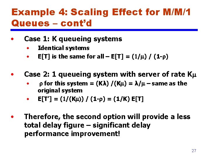
Example 4: Scaling Effect for M/M/1 Queues – cont’d • Case 1: K queueing systems • • • Case 2: 1 queueing system with server of rate Km • • • Identical systems E[T] is the same for all – E[T] = (1/m) / (1 - ) for this system = (Kλ) /(Km) = λ/m – same as the original system E[T’] = (1/(Km)) / (1 - ) = (1/K) E[T] Therefore, the second option will provide a less total delay figure – significant delay performance improvement! 27

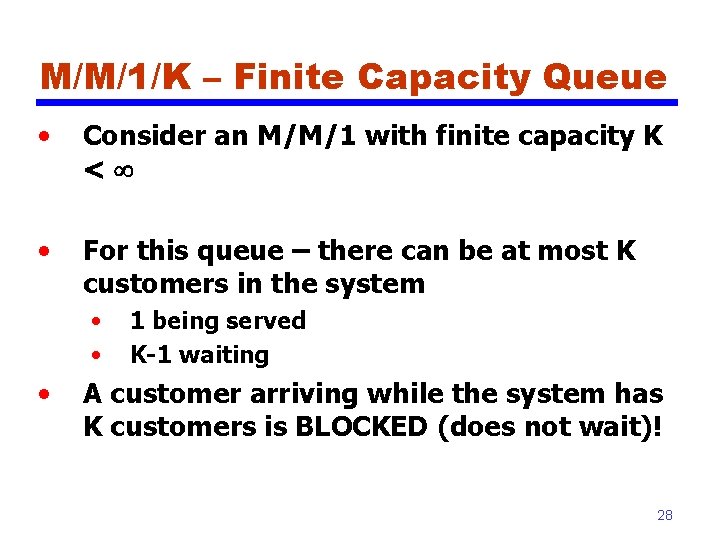
M/M/1/K – Finite Capacity Queue • Consider an M/M/1 with finite capacity K < • For this queue – there can be at most K customers in the system • • • 1 being served K-1 waiting A customer arriving while the system has K customers is BLOCKED (does not wait)! 28

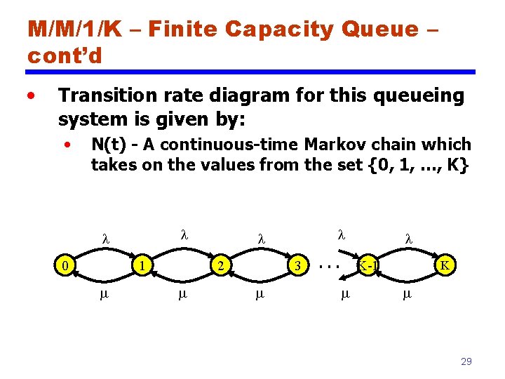
M/M/1/K – Finite Capacity Queue – cont’d • Transition rate diagram for this queueing system is given by: • N(t) - A continuous-time Markov chain which takes on the values from the set {0, 1, …, K} l l 0 1 m 2 m l l 3 m l K-1 m K m 29

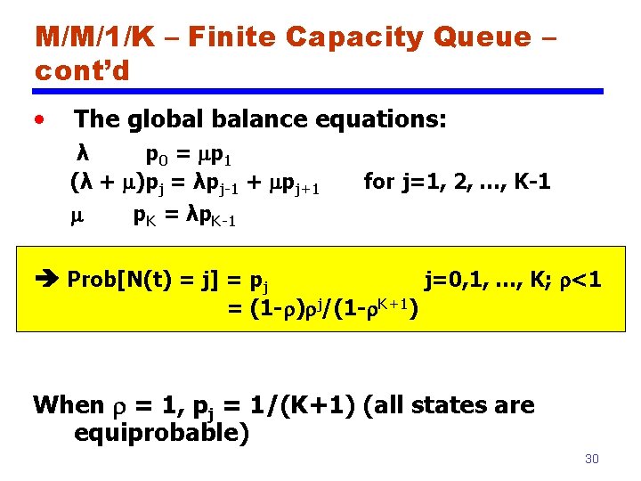
M/M/1/K – Finite Capacity Queue – cont’d • The global balance equations: λ p 0 = mp 1 (λ + m)pj = λpj-1 + mpj+1 m for j=1, 2, …, K-1 p. K = λp. K-1 Prob[N(t) = j] = pj j=0, 1, …, K; <1 = (1 - ) j/(1 - K+1) When = 1, pj = 1/(K+1) (all states are equiprobable) 30
![MM1K Mean Number of Customers Mean number of customers EN is given M/M/1/K – Mean Number of Customers • Mean number of customers, E[N] is given](https://slidetodoc.com/presentation_image_h/c513bbcaf61550d78772953cacd7eabd/image-31.jpg)
M/M/1/K – Mean Number of Customers • Mean number of customers, E[N] is given by: 31

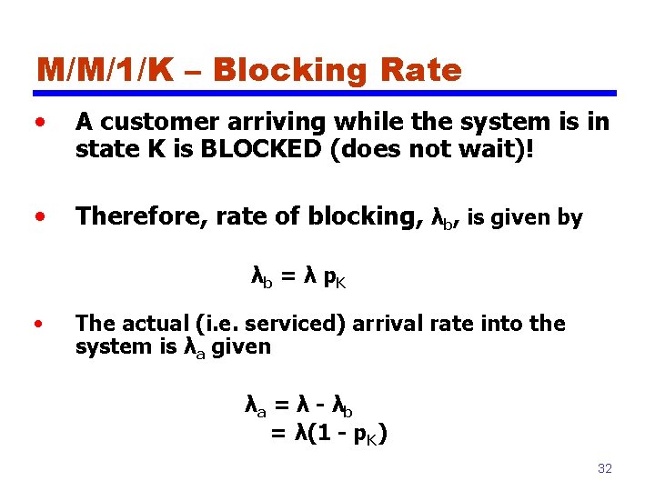
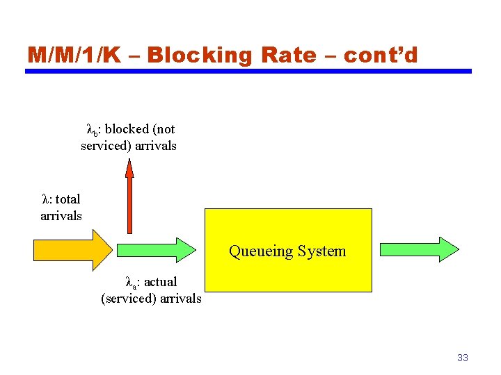
M/M/1/K – Blocking Rate • A customer arriving while the system is in state K is BLOCKED (does not wait)! • Therefore, rate of blocking, λb, is given by λ b = λ p. K • The actual (i. e. serviced) arrival rate into the system is λa given λa = λ - λb = λ(1 - p. K) 32

M/M/1/K – Blocking Rate – cont’d λb: blocked (not serviced) arrivals λ: total arrivals Queueing System λa: actual (serviced) arrivals 33
![MM1K Mean Delay The mean total delay ET is given by ET M/M/1/K – Mean Delay • The mean total delay E[T] is given by E[T]](https://slidetodoc.com/presentation_image_h/c513bbcaf61550d78772953cacd7eabd/image-34.jpg)
M/M/1/K – Mean Delay • The mean total delay E[T] is given by E[T] = E[N] / λa 34

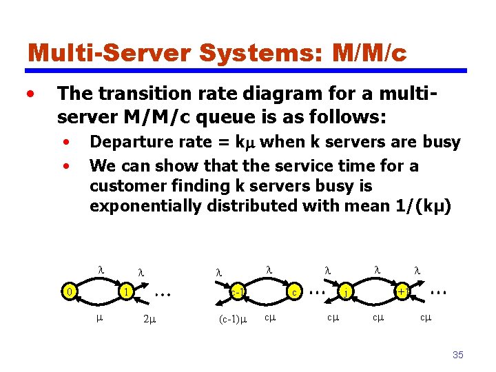
Multi-Server Systems: M/M/c • The transition rate diagram for a multiserver M/M/c queue is as follows: • • Departure rate = km when k servers are busy We can show that the service time for a customer finding k servers busy is exponentially distributed with mean 1/(kμ) l 0 l 1 m l l c-1 2 m (c-1)m c cm l l j cm l j+1 cm cm 35

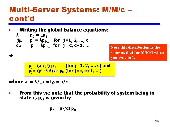
Multi-Server Systems: M/M/c – cont’d • Writing the global balance equations: λ jm cm p 0 = mp 1 pj = λpj-1 for j=1, 2, …, c pj = λpj-1 for j= c, c+1, … Note this distribution is the same as that for M/M/1 when you set c to 1. pj= (aj/j!) p 0 (for j=1, 2, …, c) and pj= ( j-c/c!) ac p 0 (for j=c, c+1, …) where a = λ/m and = a/c • From this we note that the probability of system being in state c, pc, is given by p c = ac/c! p 0 36

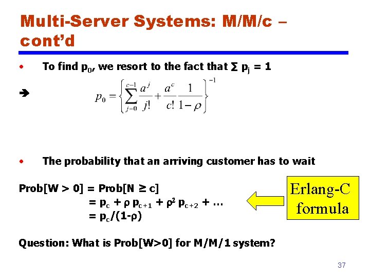
Multi-Server Systems: M/M/c – cont’d • To find p 0, we resort to the fact that ∑ pj = 1 • The probability that an arriving customer has to wait Prob[W > 0] = Prob[N ≥ c] = pc + pc+1 + 2 pc+2 + … = pc/(1 - ) Erlang-C formula Question: What is Prob[W>0] for M/M/1 system? 37

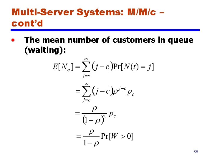
Multi-Server Systems: M/M/c – cont’d • The mean number of customers in queue (waiting): 38

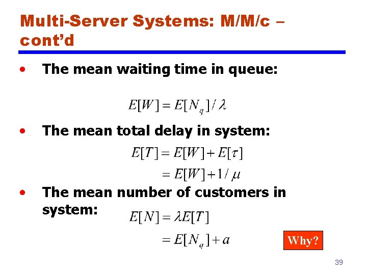
Multi-Server Systems: M/M/c – cont’d • The mean waiting time in queue: • The mean total delay in system: • The mean number of customers in system: Why? 39

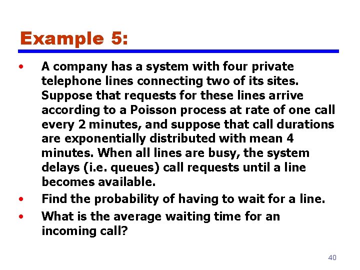
Example 5: • • • A company has a system with four private telephone lines connecting two of its sites. Suppose that requests for these lines arrive according to a Poisson process at rate of one call every 2 minutes, and suppose that call durations are exponentially distributed with mean 4 minutes. When all lines are busy, the system delays (i. e. queues) call requests until a line becomes available. Find the probability of having to wait for a line. What is the average waiting time for an incoming call? 40

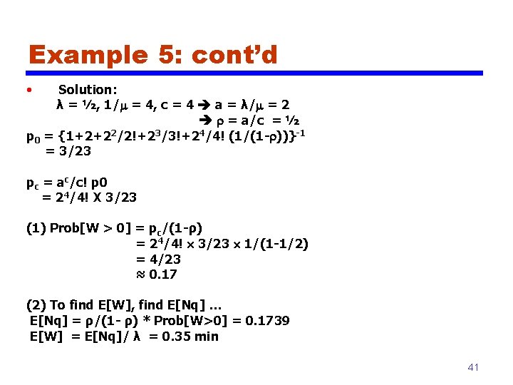
Example 5: cont’d • Solution: λ = ½, 1/m = 4, c = 4 a = λ/m = 2 = a/c = ½ p 0 = {1+2+22/2!+23/3!+24/4! (1/(1 - ))}-1 = 3/23 pc = ac/c! p 0 = 24/4! X 3/23 (1) Prob[W > 0] = pc/(1 -ρ) = 2 4/4! 3/23 1/(1 -1/2) = 4/23 ≈ 0. 17 (2) To find E[W], find E[Nq] … E[Nq] = ρ/(1 - ρ) * Prob[W>0] = 0. 1739 E[W] = E[Nq]/ λ = 0. 35 min 41

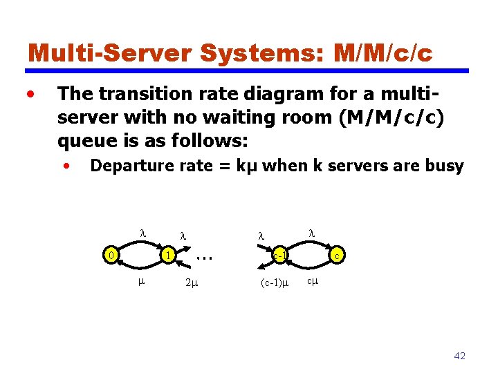
Multi-Server Systems: M/M/c/c • The transition rate diagram for a multiserver with no waiting room (M/M/c/c) queue is as follows: • Departure rate = kμ when k servers are busy l 0 l 1 m l l c-1 2 m (c-1)m c cm 42

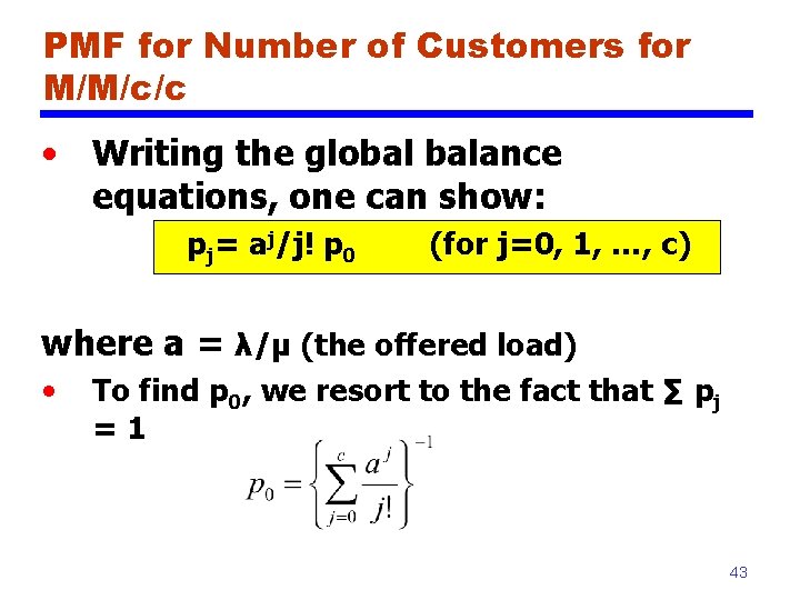
PMF for Number of Customers for M/M/c/c • Writing the global balance equations, one can show: pj= aj/j! p 0 (for j=0, 1, …, c) where a = λ/μ (the offered load) • To find p 0, we resort to the fact that ∑ pj =1 43

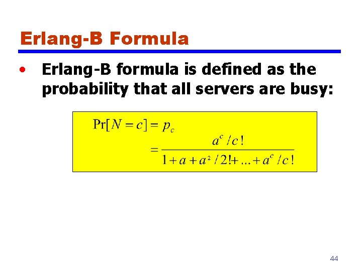
Erlang-B Formula • Erlang-B formula is defined as the probability that all servers are busy: 44

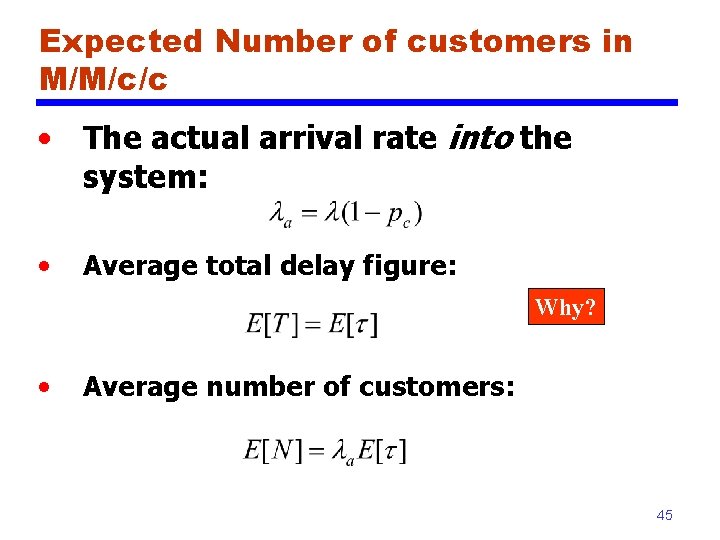
Expected Number of customers in M/M/c/c • The actual arrival rate into the system: • Average total delay figure: Why? • Average number of customers: 45

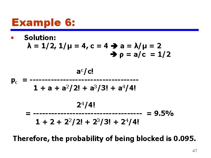
Example 6: • • A company has a system with four private telephone lines connecting two of its sites. Suppose that requests for these lines arrive according to a Poisson process at rate of one call every 2 minutes, and suppose that call durations are exponentially distributed with mean 4 minutes. When all lines are busy, the system BLOCKS the incoming call and generates a busy signal. Find the probability of being blocked. 46

Example 6: • Solution: λ = 1/2, 1/μ = 4, c = 4 a = λ/μ = 2 ρ = a/c = 1/2 a c/c! pc = ------------------1 + a 2/2! + a 3/3! + a 4/4! 2 4/4! = ------------------ = 9. 5% 1 + 22/2! + 23/3! + 24/4! Therefore, the probability of being blocked is 0. 095. 47

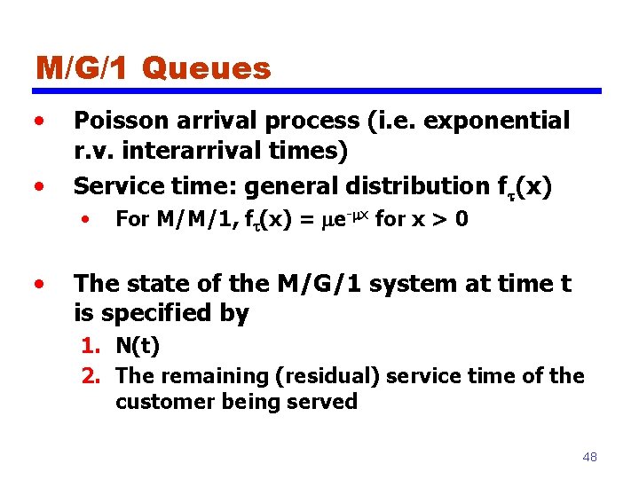
M/G/1 Queues • • Poisson arrival process (i. e. exponential r. v. interarrival times) Service time: general distribution f (x) • • For M/M/1, f (x) = me-mx for x > 0 The state of the M/G/1 system at time t is specified by 1. N(t) 2. The remaining (residual) service time of the customer being served 48

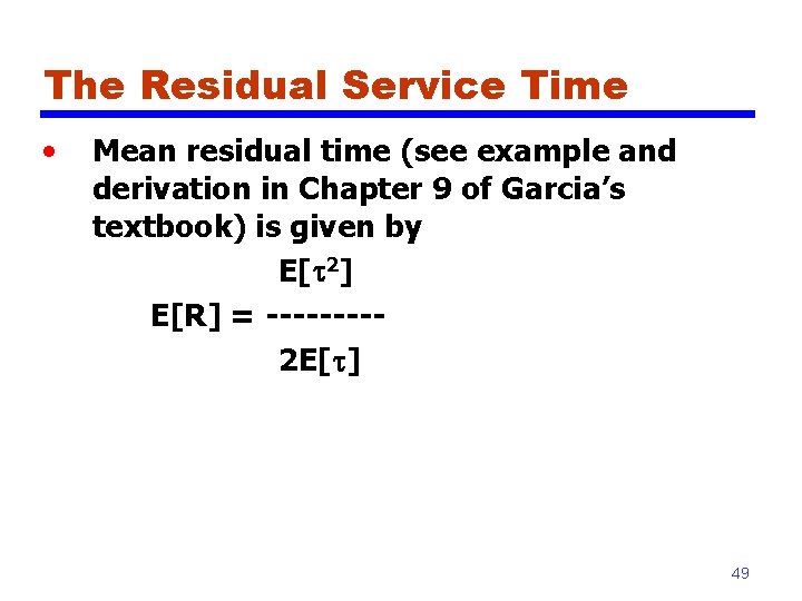
The Residual Service Time • Mean residual time (see example and derivation in Chapter 9 of Garcia’s textbook) is given by E[ 2] E[R] = ----2 E[ ] 49

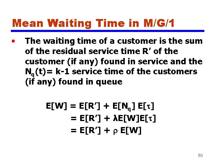
Mean Waiting Time in M/G/1 • The waiting time of a customer is the sum of the residual service time R’ of the customer (if any) found in service and the Nq(t)= k-1 service time of the customers (if any) found in queue E[W] = E[R’] + E[Nq] E[ ] = E[R’] + λE[W]E[ ] = E[R’] + E[W] 50

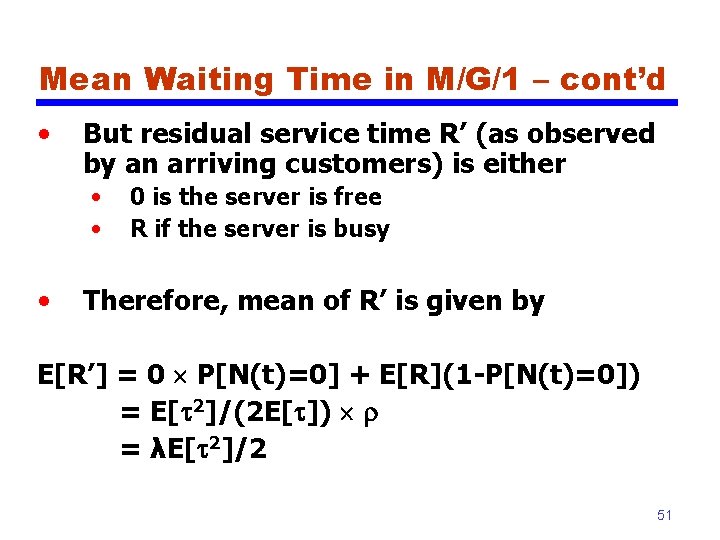
Mean Waiting Time in M/G/1 – cont’d • But residual service time R’ (as observed by an arriving customers) is either • • • 0 is the server is free R if the server is busy Therefore, mean of R’ is given by E[R’] = 0 P[N(t)=0] + E[R](1 -P[N(t)=0]) = E[ 2]/(2 E[ ]) = λE[ 2]/2 51
![Mean Waiting Time in MG1 contd Substituting back yields λE 2 EW Mean Waiting Time in M/G/1 – cont’d • Substituting back, yields λE[ 2] E[W]](https://slidetodoc.com/presentation_image_h/c513bbcaf61550d78772953cacd7eabd/image-52.jpg)
Mean Waiting Time in M/G/1 – cont’d • Substituting back, yields λE[ 2] E[W] = -----2(1 - ) λ(δ 2 +E[ ]2) = --------2(1 - ) (1 + C 2) = -------- E[ ] 2(1 - ) Note: - E[ 2] = δ 2 +E[ ]2 - C 2 = δ 2 /E[ ]2 = coefficient of variation of the service time Pollaczek-Khinchin (P-K) Mean Value Formula 52
![Mean Delay in MG1 contd The mean waiting time ET is found Mean Delay in M/G/1 – cont’d • The mean waiting time, E[T] is found](https://slidetodoc.com/presentation_image_h/c513bbcaf61550d78772953cacd7eabd/image-53.jpg)
Mean Delay in M/G/1 – cont’d • The mean waiting time, E[T] is found by adding mean service time to E[W]: E[T] = E[ ] + E[W] (1 + C 2) = E[ ] + -------- E[ ] 2(1 - ) 53
![Example 7 Problem Compare EW for MM1 and MD1 systems Answer MM1 Example 7: • Problem: Compare E[W] for M/M/1 and M/D/1 systems. • Answer: M/M/1:](https://slidetodoc.com/presentation_image_h/c513bbcaf61550d78772953cacd7eabd/image-54.jpg)
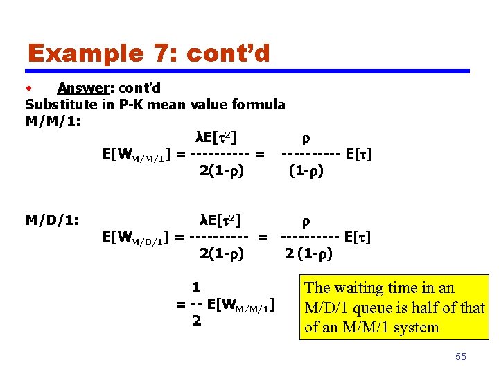
Example 7: • Problem: Compare E[W] for M/M/1 and M/D/1 systems. • Answer: M/M/1: service time, , is exponential r. v. with parameter m E[ ] = 1/m , E[ 2] = 2/m 2 , δ 2 = 1/m 2 , C 2 = 1 M/D/1: service time, , is constant with value = 1/m E[ ] = 1/m , E[ 2] = 1/m 2 , δ 2 = 0 , C 2 = 0 54

Example 7: cont’d • Answer: cont’d Substitute in P-K mean value formula M/M/1: λE[ 2] E[WM/M/1] = ---------- E[ ] 2(1 - ) M/D/1: λE[ 2] E[WM/D/1] = ---------- E[ ] 2(1 - ) 2 (1 - ) 1 = -- E[W M/M/1] 2 The waiting time in an M/D/1 queue is half of that of an M/M/1 system 55

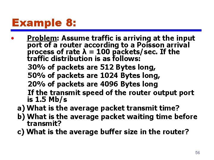
Example 8: • Problem: Assume traffic is arriving at the input port of a router according to a Poisson arrival process of rate λ = 100 packets/sec. If the traffic distribution is as follows: 30% of packets are 512 Bytes long, 50% of packets are 1024 Bytes long, 20% of packets are 4096 Bytes long If the transmit speed of the router output port is 1. 5 Mb/s a) What is the average packet transmit time? b) What is the average packet waiting time before transmit? c) What is the average buffer size in the router? 56
![Example 8 contd Solution a Average packet size EL 0 3 512 Example 8: cont’d • Solution: a) Average packet size, E[L] = 0. 3 512](https://slidetodoc.com/presentation_image_h/c513bbcaf61550d78772953cacd7eabd/image-57.jpg)
Example 8: cont’d • Solution: a) Average packet size, E[L] = 0. 3 512 + 0. 5 1024 + 0. 2 4096 = 1484. 8 Bytes average transmit time = E[L]/R = 1484. 8 8/1. 5 106 = 0. 0079 sec b) E[L 2] = 0. 3 (512 8)2 + 0. 5 (1024 8)2 + 0. 2 x(4096 8)2 = 2. 5334 e+008 Bits 2 E[ 2] = E[L 2]/R 2 = 1. 1259 e-004 sec 2 ρ = λ E[ ] = 0. 7919 E[W] = (½) λ E[ 2] /(1 -ρ) = 0. 0271 sec c) E[Nq] = λ E[W] = 2. 705 packet 57