KERNELS AND PERCEPTRONS The perceptron x is a

KERNELS AND PERCEPTRONS

The perceptron x is a vector y is -1 or +1 instance xi A B ^ yi ^ Compute: yi = sign(vk. xi ) If mistake: vk+1 = vk + yi xi yi u Depends on how easy the learning problem is, not dimension of vectors x +x 2 v 2 >γ Fairly intuitive: • “Similarity” of v to u looks like (v. u)/|v. v| • (v. u) grows by >= γafter mistake • (v. v) grows by <= R 2 v 1 -u 2γ 2

The kernel perceptron A instance xi B ^ yi yi ^ Compute: yi = sign(vk. xi ) If mistake: vk+1 = vk + yi xi Mathematically the same as before … but allows use of the kernel trick 3

The kernel perceptron A instance xi B ^ yi yi ^ Compute: yi = vk. xi If mistake: vk+1 = vk + yi xi Mathematically the same as before … but allows use of the “kernel trick” Other kernel methods (SVM, Gaussian processes) aren’t constrained to limited set (+1/-1/0) of weights on the K(x, v) values. 4

Some common kernels • Linear kernel: • Polynomial kernel: • Gaussian kernel: • More later…. 5

Kernels 101 • Duality – and computational properties – Reproducing Kernel Hilbert Space (RKHS) • Gram matrix • Positive semi-definite • Closure properties 6

Explicitly map from x to φ(x) – i. e. to the point corresponding to x in the Hilbert space Kernels 101 Implicitly map from x to φ(x) by changing the kernel function K • Duality: two ways to look at this Two different computational ways of getting the same behavior 7

Kernels 101 • Duality • Gram matrix: K(x, x’) = K(x’, x) Gram matrix is symmetric K: kij = K(xi, xj) 8

Kernels 101 • Duality • Gram matrix: K: kij = K(xi, xj) K(x, x’) = K(x’, x) Gram matrix is symmetric K is “positive semi-definite” … z. T K z >= 0 for all z Fun fact: Gram matrix positive semi-definite K(xi, xj)=φ(xi), φ(xj) for some φ Proof: φ(x) uses the eigenvectors of K to represent x 9

HASH KERNELS AND “THE HASH TRICK” 10

Question • Most of the weights in a classifier are – small and not important – So we can use the “hash trick” 11

12

The hash trick as a kernel • Usually we implicitly map from x to φ(x) – All computations of learner are in terms of K(x, x’) = <φ(x), φ(x’) > – Because φ(x) is large • In this case we explicitly map from x to φ(x) – φ(x) is small

Some details Slightly different hash to avoid systematic bias m is the number of buckets you hash into (R in my discussion) 14

Some details Slightly different hash to avoid systematic bias m is the number of buckets you hash into (R in my discussion) 15

Some details I. e. – a hashed vector is probably close to the original vector 16

Some details I. e. the inner products between x and x’ are probably not changed too much by the hash function: a classifier will probably still work 17

Some details 18

The hash kernel: implementation • One problem: debugging is harder – Features are no longer meaningful – There’s a new way to ruin a classifier • Change the hash function • You can separately compute the set of all words that hash to h and guess what features mean – Build an inverted index h w 1, w 2, …, 19

ADAPTIVE GRADIENTS

Motivation • What’s the best learning rate? – If a feature is rare, but relevant, it should be high, else learning will be slow • Regularization makes this better/worse? – But then you could overshoot the local minima when you train

Motivation • What’s the best learning rate? – Depends on typical gradient for a feature • Small fast rate • Large slow rate – Sadly we can’t afford to ignore rare features • We could have a lot of them

Motivation • What’s the best learning rate? – Let’s pretend our observed gradients are from a zero-mean Gaussian and find variances, then scale dimension j by sd(j)-1

Motivation • What’s the best learning rate? – Let’s pretend our observed gradients are from a zero-mean Gaussian and find variances, then scale dimension j by sd(j)-1 – Ignore co-variances for efficiency

Motivation • What’s the best learning rate? – Let’s pretend our observed gradients are from a zero-mean Gaussian and find variances, then scale dimension j by sd(j)-1 – Ignore co-variances for efficiency

Adagrad Gradient at time τcovariances η= 1 is usually ok

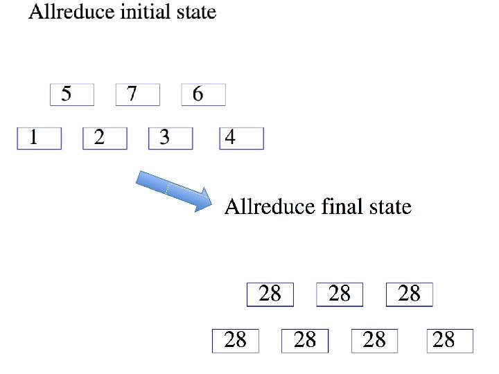
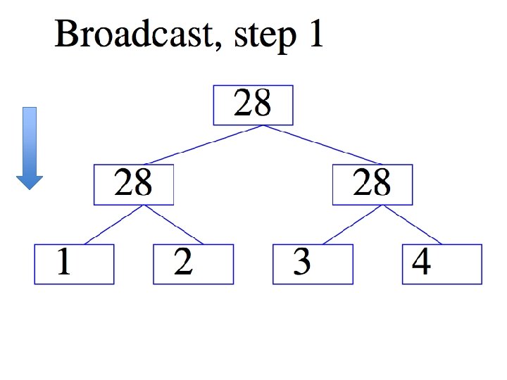
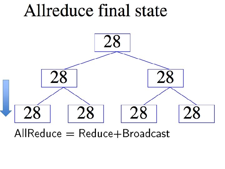
ALL-REDUCE

Introduction • Common pattern: – do some learning in parallel MAP – aggregate local changes from each processor • to shared parameters – distribute the new shared parameters ALLREDUCE • back to each processor – and repeat…. • All. Reduce implemented in MPI, recently in VW code (John Langford) in a Hadoop/compatible scheme

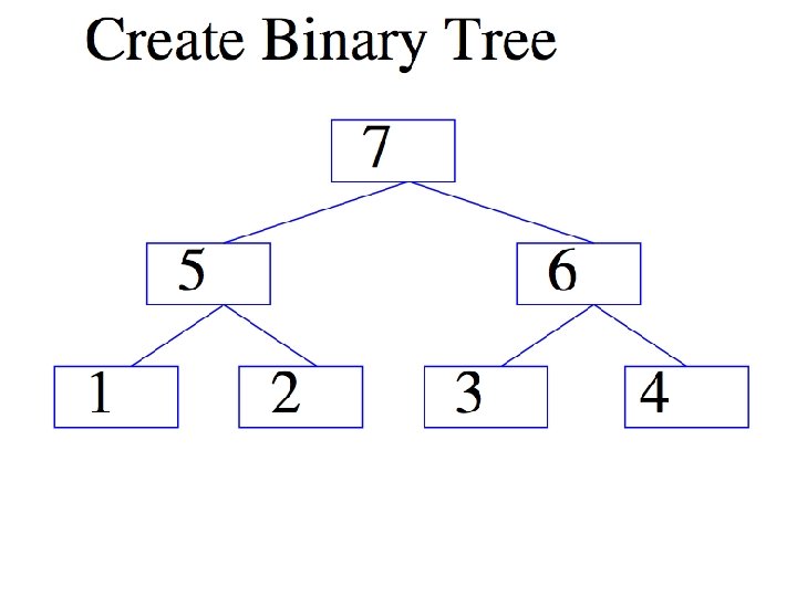
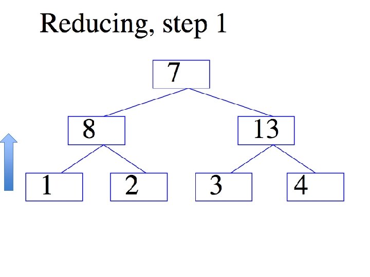
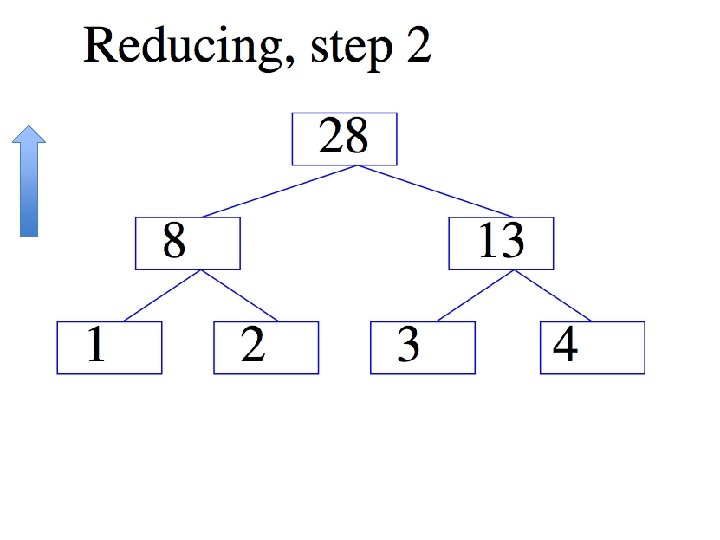
Gory details of VW Hadoop-All. Reduce • Spanning-tree server: – Separate process constructs a spanning tree of the compute nodes in the cluster and then acts as a server • Worker nodes (“fake” mappers): – Input for worker is locally cached – Workers all connect to spanning-tree server – Workers all execute the same code, which might contain All. Reduce calls: • Workers synchronize whenever they reach an all -reduce

Hadoop All. Reduce don’t wait for duplicate jobs

Second-order method - like Newton’s method

2 24 features ~=100 nonzeros/example 2. 3 B examples example is user/page/ad and conjunctions of these, positive if there was a click-thru on the ad

50 M examples explicitly constructed kernel 11. 7 M features 3, 300 nonzeros/example old method: SVM, 3 days: reporting time to get to fixed test error