k r o w h t r a

k r o w h t r a E Cross Section and Borrow Pit Methods

This lecture covers: • Readings: 26 -1 to 26 -6, 26 -8 to 26 -10. • Figures: 26 -1 to 26 -4, 26 -6, and 26 -7 • Plate B-5 page 893, and B-2 page 890 • Examples: 26 -1 and 26 -3

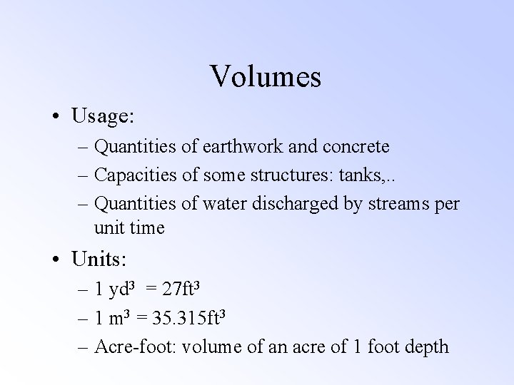
Volumes • Usage: – Quantities of earthwork and concrete – Capacities of some structures: tanks, . . – Quantities of water discharged by streams per unit time • Units: – 1 yd 3 = 27 ft 3 – 1 m 3 = 35. 315 ft 3 – Acre-foot: volume of an acre of 1 foot depth

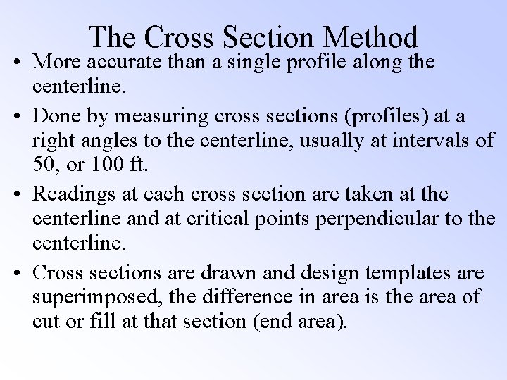
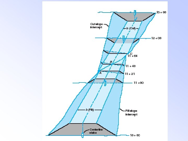
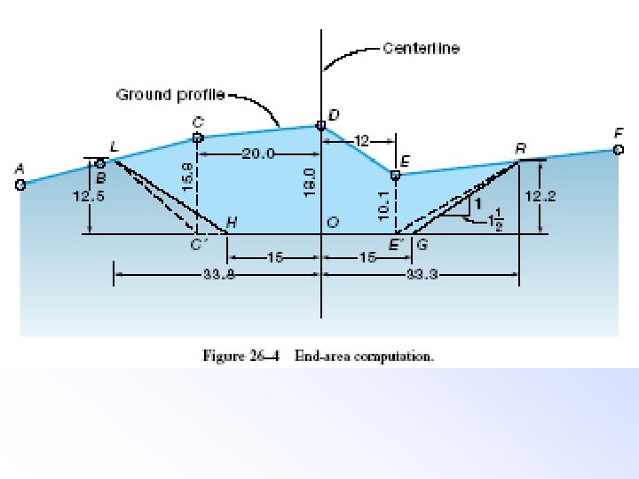
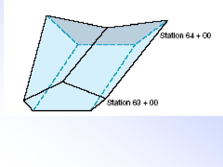
The Cross Section Method • More accurate than a single profile along the centerline. • Done by measuring cross sections (profiles) at a right angles to the centerline, usually at intervals of 50, or 100 ft. • Readings at each cross section are taken at the centerline and at critical points perpendicular to the centerline. • Cross sections are drawn and design templates are superimposed, the difference in area is the area of cut or fill at that section (end area).

• End areas can be cut, fill, or transition (both). • Use the areas to compute volumes, knowing the distance between the sections. • The whole work can be done with photogrammetry and a computer software.

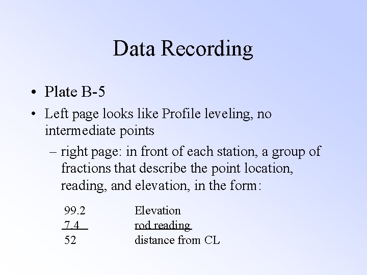
Data Recording • Plate B-5 • Left page looks like Profile leveling, no intermediate points – right page: in front of each station, a group of fractions that describe the point location, reading, and elevation, in the form: 99. 2 7. 4 52 Elevation rod reading distance from CL

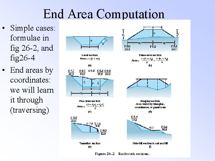
End Area Computation • Simple cases: formulae in fig 26 -2, and fig 26 -4 • End areas by coordinates: we will learn it through (traversing)

End Area Computation • Simple cases: formulae in fig 27 -2, and fig 27 -4

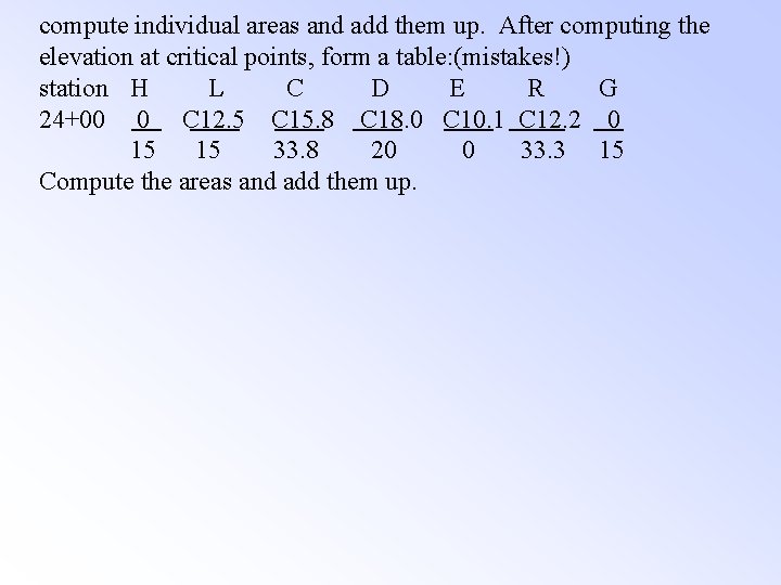
compute individual areas and add them up. After computing the elevation at critical points, form a table: (mistakes!) station H L C D E R G 24+00 0 C 12. 5 C 15. 8 C 18. 0 C 10. 1 C 12. 2 0 15 15 33. 8 20 0 33. 3 15 Compute the areas and add them up.

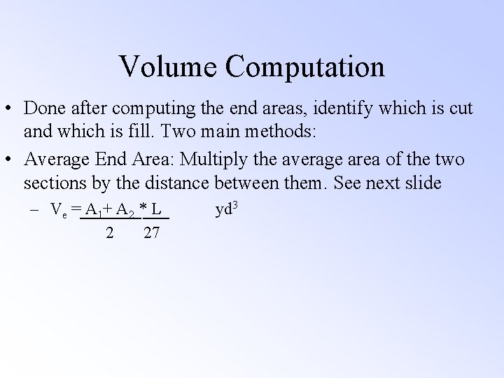
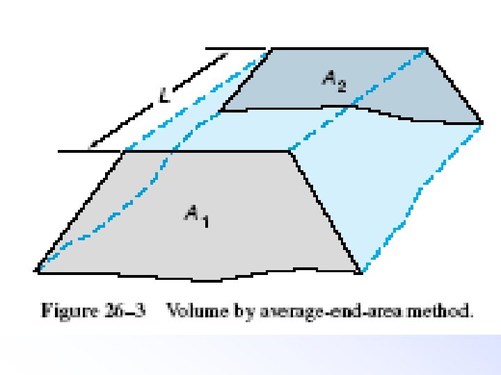
Volume Computation • Done after computing the end areas, identify which is cut and which is fill. Two main methods: • Average End Area: Multiply the average area of the two sections by the distance between them. See next slide – Ve = A 1+ A 2 * L 2 27 yd 3

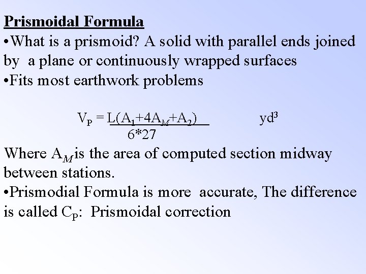
Prismoidal Formula • What is a prismoid? A solid with parallel ends joined by a plane or continuously wrapped surfaces • Fits most earthwork problems VP = L(A 1+4 AM+A 2) 6*27 yd 3 Where AM is the area of computed section midway between stations. • Prismodial Formula is more accurate, The difference is called CP: Prismoidal correction

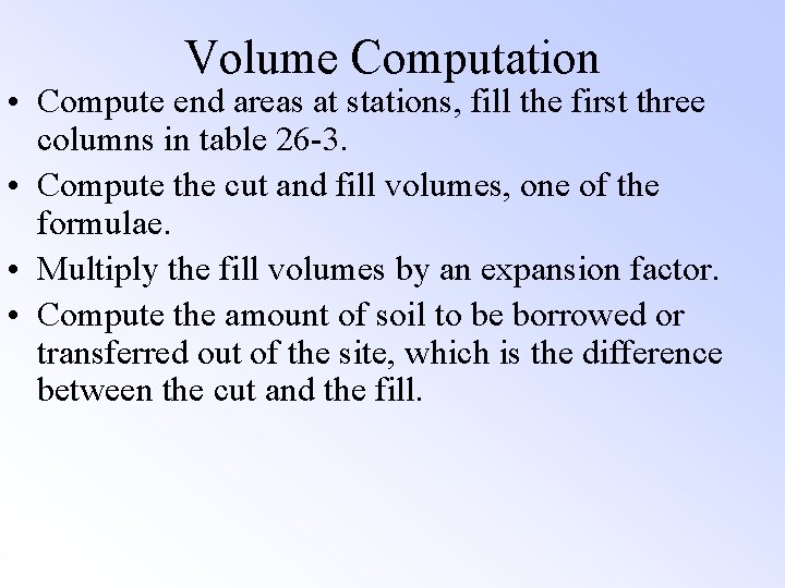
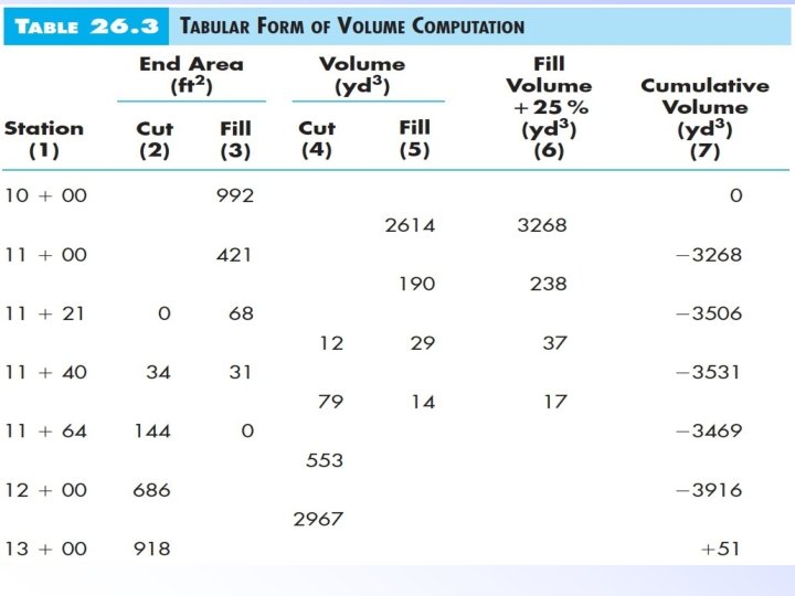
Volume Computation • Compute end areas at stations, fill the first three columns in table 26 -3. • Compute the cut and fill volumes, one of the formulae. • Multiply the fill volumes by an expansion factor. • Compute the amount of soil to be borrowed or transferred out of the site, which is the difference between the cut and the fill.

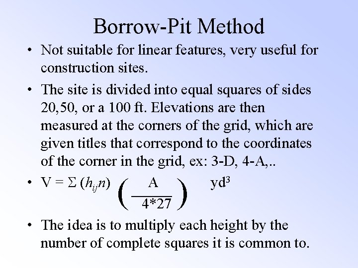
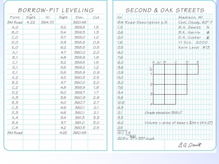
Borrow-Pit Method • Not suitable for linear features, very useful for construction sites. • The site is divided into equal squares of sides 20, 50, or a 100 ft. Elevations are then measured at the corners of the grid, which are given titles that correspond to the coordinates of the corner in the grid, ex: 3 -D, 4 -A, . . • V = (hijn) A yd 3 4*27 • The idea is to multiply each height by the number of complete squares it is common to. ( )

Plate B. 2

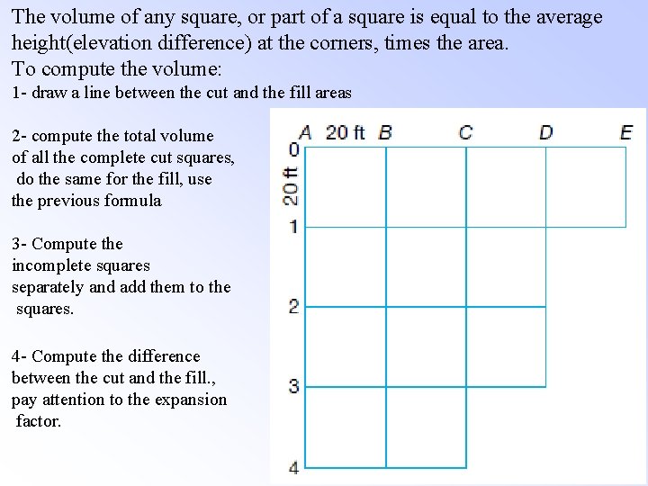
The volume of any square, or part of a square is equal to the average height(elevation difference) at the corners, times the area. To compute the volume: 1 - draw a line between the cut and the fill areas 2 - compute the total volume of all the complete cut squares, do the same for the fill, use the previous formula 3 - Compute the incomplete squares separately and add them to the squares. 4 - Compute the difference between the cut and the fill. , pay attention to the expansion factor.

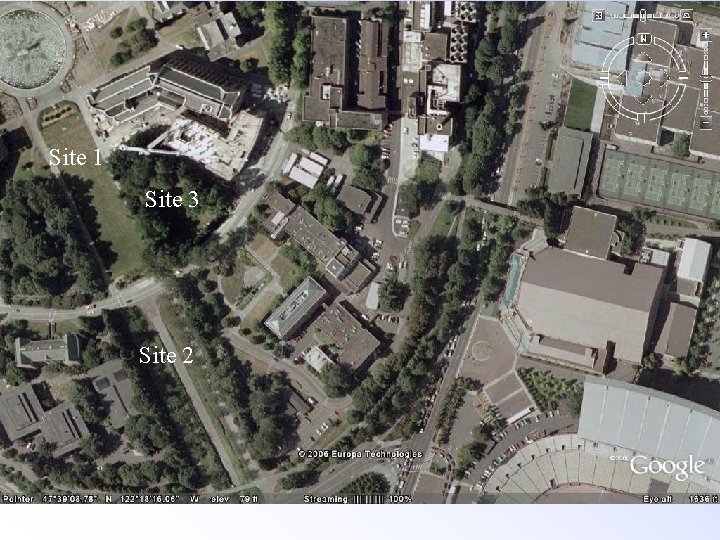
Site 1 Site 3 Site 2

PROJECT 1 Instructions

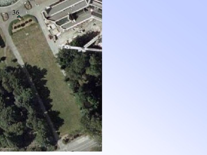
36

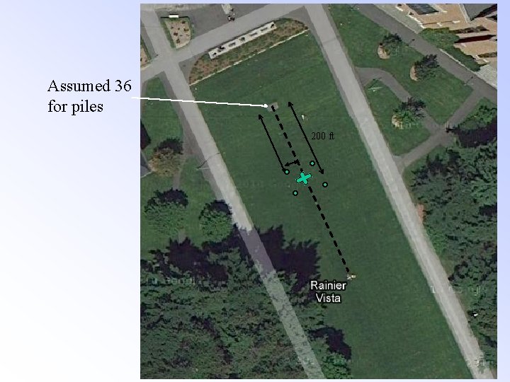
Assumed 36 for piles 200 ft

20

C D B A