JPEG Introduction n JPEG Joint Photographic Experts Group

JPEG

Introduction n JPEG (Joint Photographic Experts Group) n Basic Concept Data compression is performed in the frequency domain. Low frequency components are retained. High frequency components are truncated

JPEG System Overview n The JPEG is a transform coding scheme. Its encoding process can be separated into 3 stages: Color Transform Discrete Cosine Transform Quantization Bitstream Formation

Color Transform Process the data in blocks of 8× 8 samples n Convert RGB into Luminance (Y) and Chrominance (Cr and Cb). n Use half resolution for Chrominance (because eye is more sensitive to Luminance) n

Discrete Cosine Transform n Transform each block of 8× 8 samples into 64 DCT coefficients – energy tends to be concentrated into a few significant coefficients

Quantization (I) Divide each DCT coefficient by an integer, discard remainder n Typically, a few non-zero coefficients are left. n

Quantization (II)

DCT Transform n The JPEG is based on the 8 × 8 DCT. n To use the DCT , we first divide an image into non-overlapping 8 × 8 blocks. n Let x(n, m), 0≦n, m≦ 7, be the pixel values in the block. n Let X(u, v), 0≦u, v≦ 7, be the DCT coefficients.

The X(u, v) and x(n, m) are related by where and N=8

Quantization In the JPEG, each of the 64 resulting DCT coefficients is quantized by an uniform scalar quantizer according to the following equation: where Xq(u, v) is the quantized coefficient and

is the quantization table.

Note that Q should be the same at the encoder and decoder. Given Xq(u, v) and Q(u, v), 0≦ u, v≦ 7, the dequantized DCT coefficients Xr(u, v), 0≦ u, v≦ 7, are then obtained by Xr(u, v) = Xq(u, v) Q(u, v)

Example n Original Image block x(m, n) 79 75 79 82 82 86 94 94 76 78 76 82 83 86 85 94 72 75 67 78 80 78 74 82 74 76 75 75 86 80 81 79 73 70 75 67 78 78 79 85 69 63 68 69 75 78 82 80 76 76 71 71 67 79 80 83 72 77 78 69 75 75 78 78

n DCT coefficients of the image block X(u, v) 619 -29 8 2 1 -3 0 1 22 -6 -4 0 7 0 -2 -3 11 0 5 -4 -3 4 0 -3 2 -10 5 0 0 7 3 2 6 2 -1 -1 -3 0 0 8 1 2 0 2 -2 -2 -8 -2 -4 1 2 1 -1 1 -3 1 5 -2 1 -1 1 -3

n Quantization table Q(u, v) 16 11 10 16 24 40 51 61 12 12 14 19 26 58 60 55 14 13 16 24 40 57 69 56 14 17 22 29 51 87 80 62 18 22 37 56 68 109 103 77 24 35 55 64 81 104 113 92 49 64 78 87 103 121 120 101 72 92 95 98 112 100 103 99

n Quantized DCT coefficients Xq(u, v) 39 -3 1 0 0 0 2 -1 0 0 0 0 0 0 0 0 0 0 0 0 0 0 1.

n Dequantized DCT coefficients Xr(u, v) 624 -33 10 0 0 24 -12 0 0 0 14 0 0 0 0 -17 0 0 0 0 0 0 0 0 0 0

n Reconstructed image block 74 75 77 80 85 91 95 98 77 77 78 79 82 86 89 91 78 77 77 77 78 81 83 84 74 74 76 78 81 82 69 69 70 72 75 78 82 84 68 68 69 71 75 79 82 85 73 73 72 73 75 77 80 81 78 77 76 75 74 75 76 77

n Error block 5 0 2 2 -3 -5 -1 -4 -1 1 -2 3 1 0 -4 1 -6 -2 -10 1 2 -3 -9 -2 0 2 1 1 10 2 0 -3 4 1 5 -5 3 0 -3 1 1 -5 -1 -2 0 -1 0 -5 3 3 -1 -2 -8 2 0 2 -6 1 0 2 1

Bitstream Formation Here we use the Huffman code to form bitstream representing the quantized DCT coefficients.

Before performing the Huffman coding, all the quantized coefficients are separated into two groups: (1)DC coefficient: Xq(0, 0) (2)AC coefficients: Xq(u, v), u≠ 0 or v≠ 0 These two groups are encoded independently.

DC coefficient The encoding of the DC coefficient is based on the DIFFf value , defined as DIFFf = Xqf(0, 0)-Xqf-1(0, 0) where Xqf(0, 0) = The DC coefficient of the current block. Xqf-1(0, 0) = The DC coefficient of the previous block.

The DIFFf values are classified into 12 classes (Table 1). Class 0 1 2 3 4 5 6 7 8 9 10 11 DIFFf value 0 -1, 1 -3, -2, 2, 3 -7, …, -4, 4, …, 7 -15, …, -8, 8, …, 15 -31, …, -16, …, 31 -63, …, -32, …, 63 -127, …, -64, …, 127 -255, . . , -128, …, 255 -511, …, -256, …, 511 -1023, …, -512, …, 1023 -2047, . . , -1024, …, 2047 TABLE 1

The Huffman code representing each class is shown in Table 2. Class 0 1 2 3 4 5 6 7 8 9 10 11 Codeword 00 011 100 101 110 11110 1111110 111111110 TABLE 2

When DIFFf class 0, DIFFf is represented by codeword 00. When DIFFf classes 1 -11 , the representation of DIFFf consists of two parts:

The Extra Bits can be expressed in the following form: Extra Bits = Sign bit + Amplitude When DIFFf > 0, Sign bit = 1 When DIFFf < 0, Sign bit = 0

When DIFFf > 0: Amplitude=Lower-order bit of DIFFf (MSB is not include. ) When DIFFf < 0: Amplitude = 1’s complement of lower-order bits of |DIFFf |

Example If DIFFf = 5 , then it is represented as If DIFFf = -5, then it is represented as

AC coefficients The Huffman coding of the AC coefficients can be separated into three stages: Stage 1: Zig. Zag ordering of AC coefficients. Stage 2: Run/Size Representation of Nonzero AC coefficients. Stage 3: Huffman encoding based on the Run/Size Representation.

Zig-zag Ordering

Run/Size Representation Because many AC coefficients become zero after quantization, runs of zeros along the zigzag scan are identified and compacted.

Each nonzero AC coefficientis descibed by a composite R/S, where R(Run) is a 4 -bit zero-run from the previous non-zero value, and S(Size) represents the size of the non-zero AC coefficient.

The size can be separated into 10 classes as shown in Table 3. Class 1 2 3 4 5 6 7 8 9 10 AC coefficients -1, 1 -3, -2, 2, 3 -7, . . , -4, 4, . . , 7 -15, …, -8, 8, …, 15 -31, …, -16, …, 31 -63, …, -32, …, 63 -127, …, -64, …, 127 -255, …, -128, …, 255 -511, …, -256, …, 511 -1023, …, -512, …, 1023 TABLE 3

Huffman Encoding A Huffman table has been generated for each composite R/S. The Huffman encoding process of the AC coefficients is based on the table. The additional bits to the Huffman codes are the same as those for coding the DC coefficients.

There are two special cases that describe some attention : Case 1 : all the remaining coefficients along the zigzag scan are zero. In this case, we set R/S =x’ 00’, which is coded as an EOB code of 1010.

Case 2 : zero-run are greater than 16. In this case , we set R/S = x’F 0’(15 zeroruns and 1 zero value). Therefore 16 zero-runs are coded. The same procedure is repeated until the length of zero-runs is less than 16.

Example Consider the Xq matrix shown below: After the zig-zag ordering process , we have (39 -3 2 1 -1 1 0 0 0 -1 EOB)

To encode 39 , we first have to compute DIFFf , Note that Xqf(0, 0) = 39 , Assume Xqf-1(0, 0) = 34. Then DIFFf = 5 , From the previous example, We conclude that 39 can be encoded as 100101

The first AC coefficient is – 3. The R and S values for – 3 is R=0 and S=2 , respectively. The corresponding Huffman code is 01. Consequently, -3 is encoded as Proceed in the similar fashion , we have (100101/0100/0110/001/000/001/1111010 0/1010)

Note that the last nonzero coefficient – 1 has R=5 and S=1. The Huffman code therefore is 1111010. Consequently, -1 is encode as A total of 35 bits are needed to deliver this block. The bit rate for this block is

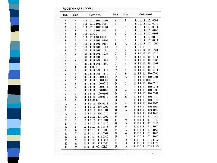
Run/Size Table

Discussions n The major drawbacks of JPEG are: – The algorithm may have block artifact. – It is difficult to perform accurate control. – It is sensitive to transmission errors.