JOURNAL CLUB General Formulation for Quantitative Gfactor Calculation

JOURNAL CLUB: “General Formulation for Quantitative G-factor Calculation in GRAPPA Reconstructions” Breuer, Griswold, et al. Research Center Magnetic Resonance Bavaria, Wurzburg, Germany Mar 31, 2014 Jason Su

Motivation • GRAPPA is becoming the dominant form of parallel imaging – Creating reliable g-factor maps is an important tool to have – Allows the evaluation and optimization of different acquisition schemes (CAIPIRINHA or even just how to choose Ry, Rz) • In our studies, we are beginning to wonder what is an acceptable level of acceleration, esp. for visualizing thalamus – G-factor is a critical quantity for this analysis

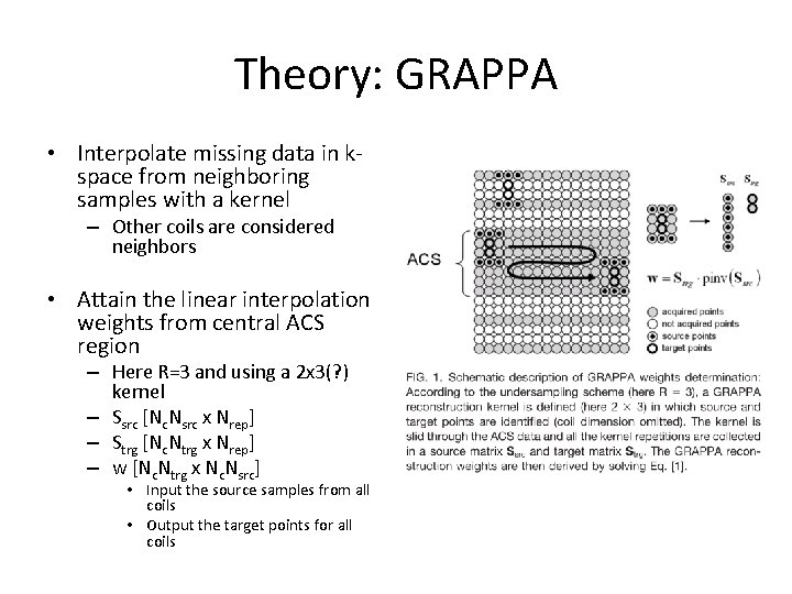
Theory: GRAPPA • Interpolate missing data in kspace from neighboring samples with a kernel – Other coils are considered neighbors • Attain the linear interpolation weights from central ACS region – Here R=3 and using a 2 x 3(? ) kernel – Ssrc [Nc. Nsrc x Nrep] – Strg [Nc. Ntrg x Nrep] – w [Nc. Ntrg x Nc. Nsrc] • Input the source samples from all coils • Output the target points for all coils

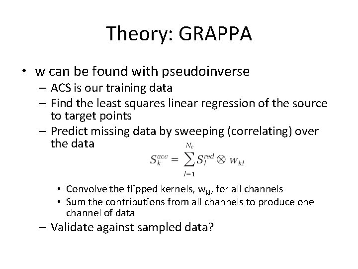
Theory: GRAPPA • w can be found with pseudoinverse – ACS is our training data – Find the least squares linear regression of the source to target points – Predict missing data by sweeping (correlating) over the data • Convolve the flipped kernels, wkl, for all channels • Sum the contributions from all channels to produce one channel of data – Validate against sampled data?

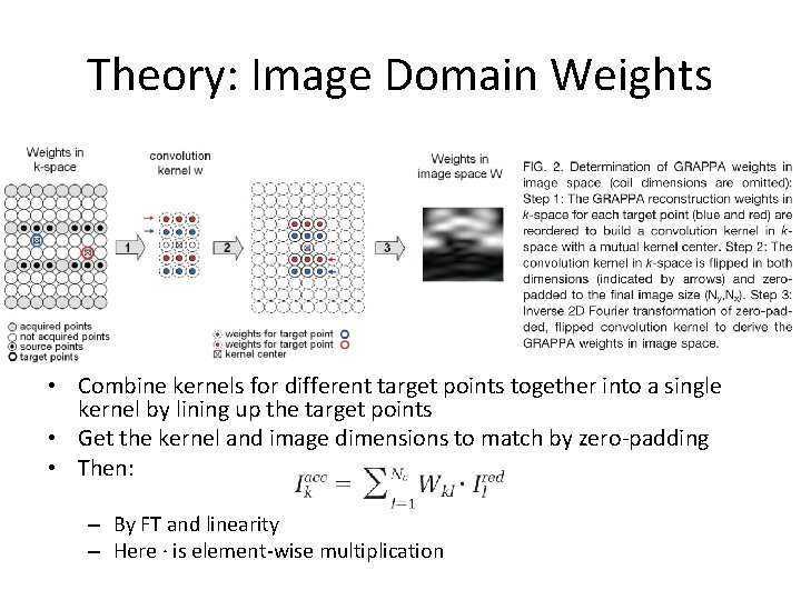
Theory: Image Domain Weights • Combine kernels for different target points together into a single kernel by lining up the target points • Get the kernel and image dimensions to match by zero-padding • Then: – By FT and linearity – Here · is element-wise multiplication

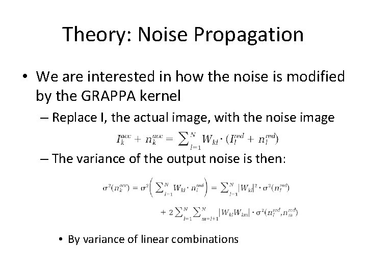
Theory: Noise Propagation • We are interested in how the noise is modified by the GRAPPA kernel – Replace I, the actual image, with the noise image – The variance of the output noise is then: • By variance of linear combinations

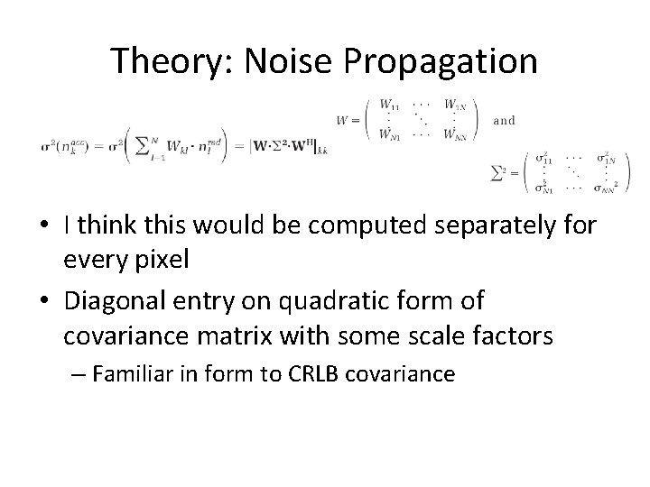
Theory: Noise Propagation • I think this would be computed separately for every pixel • Diagonal entry on quadratic form of covariance matrix with some scale factors – Familiar in form to CRLB covariance

Theory: G-factor • The g-factor for a coil image • Computed pixel-wise to obtain the whole map

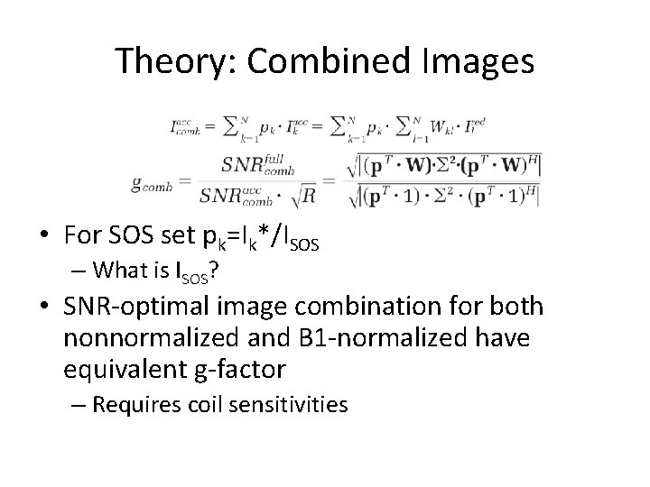
Theory: Combined Images • For SOS set pk=Ik*/ISOS – What is ISOS? • SNR-optimal image combination for both nonnormalized and B 1 -normalized have equivalent g-factor – Requires coil sensitivities

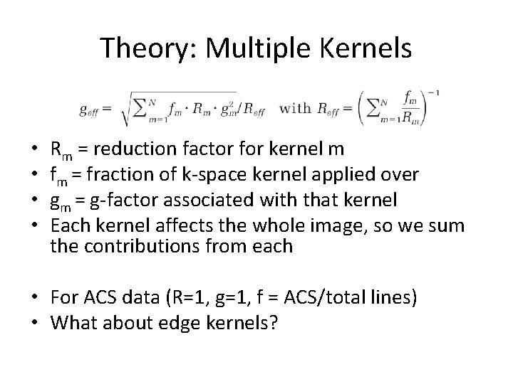
Theory: Multiple Kernels • • Rm = reduction factor for kernel m fm = fraction of k-space kernel applied over gm = g-factor associated with that kernel Each kernel affects the whole image, so we sum the contributions from each • For ACS data (R=1, g=1, f = ACS/total lines) • What about edge kernels?

Methods • Siemens 1. 5 T • 2 D Phantom – TE/TR = 7. 1/40 ms, α=30 deg. , bw=100 Hz, 256 x 256 – Noise only image with α=0 to measure noise correlation – R = [2, 3, 4] • 3 D In Vivo – MPRAGE: TE/TR = 4. 38/1350 ms, TR=800 ms, α=15 deg. , bw=180 Hz, 256 x 192 x 160 – Noise only image with α=0 – Rectangular and CAIPIRINHA sampling, R=2 x 2 • 3 x 3 x 3 kernel with 24 x 32 ACS block • Simulated non-cartesian GRAPPA – Variable density – PROPELLER, R = [2, 3, 4] • Validation against pseudomultiple replica

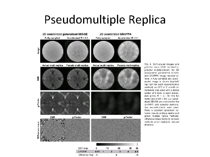
Pseudomultiple Replica • Generate 300+ artificial images by adding bootstrapped noise – Collected noise images are randomly reordered and added to the acquired coil data • Compare analytic g-factor to simulated gfactor

Pseudomultiple Replica

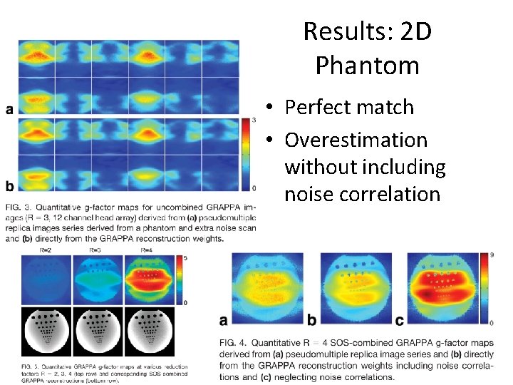
Results: 2 D Phantom • Perfect match • Overestimation without including noise correlation

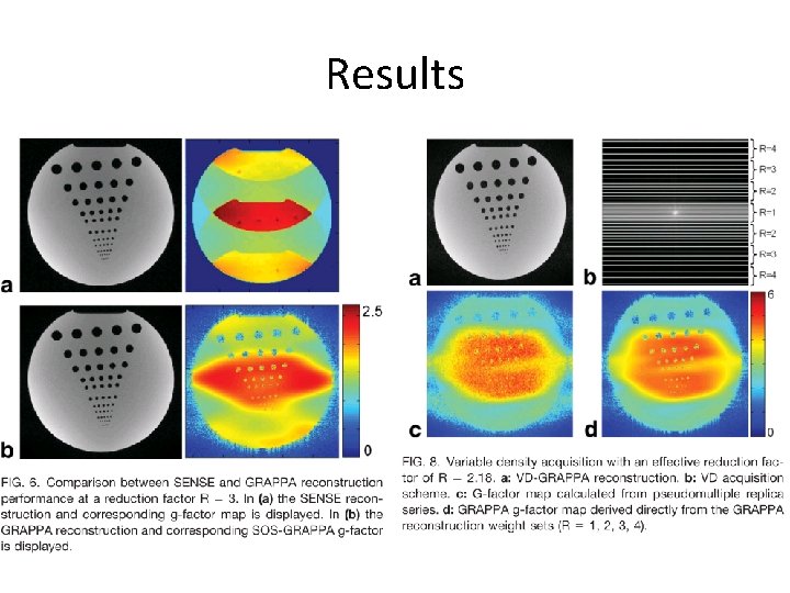
Results

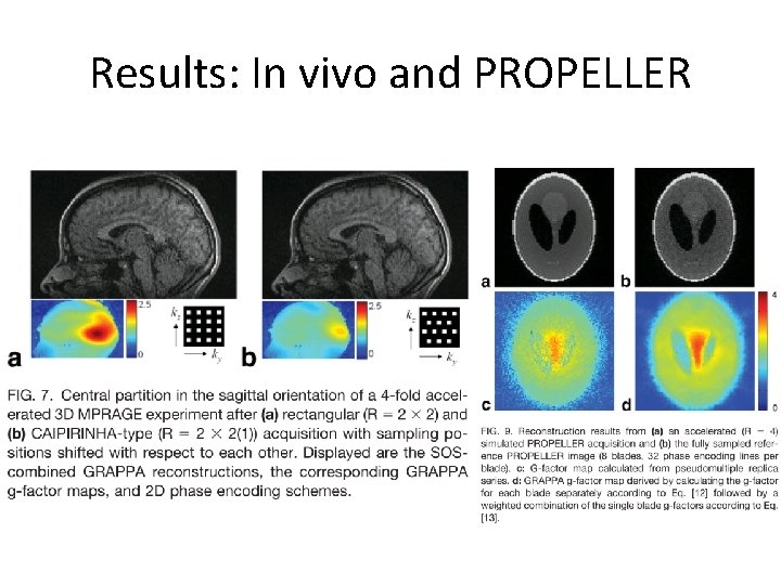
Results: In vivo and PROPELLER

Discussion • Can be used to identify the optimal reconstruction kernel, acceleration factor, sampling scheme • For multiple kernels: – Can treat kernels that share source points as having uncorrelated noise – Why?