Joint UNCTADUNECA Seminar on Regional and Global Value

Joint UNCTAD-UNECA Seminar on Regional and Global Value Chains in Services and Trade in Value Added: Quantitative Methodology Ben Shepherd, Principal, Developing Trade Consultants. 1

Key Takeaways 1. Calculating trade in value added requires a lot of data and hard work, and a little math. 2. The basic ingredients are trade data and IO tables, which are then linked together to produce a harmonized MRIO. 3. The algebra involves basic input-output relations and the Leontief inverse, which have been well understood since the 1950 s but only recently applied to trade. 4. Working with a “toy” model helps fix ideas and get the intuition straight, before moving to real data. 5. Knowledge of a statistical package is necessary to produce the full matrix of value added by origin, but once this is available, aggregate results can in theory be produced using Excel (with a bit of work and willingness to manipulate 20, 000 data points). 6. UNCTAD has produced helpful indicators using Eora for 190 countries, which participants should be familiar with. But to look at services RVCs and GVCs specifically, more detail is required: so we will learn how to calculate the full matrix and work up from there. 2

Outline 1. Measuring Trade in Value Added: Theory 2. Measuring Trade in Value Added: Application 3. Making the Data ”Talk” 4. What do the Data Say about Tourism Value Chains in Ethiopia? 3

1. Measuring Trade in Value Added: Theory 1. Start by considering how to construct an IO system for a single country, so leave trade to one side. 2. Examine the elements of the system, and the operations performed to derive quantities of interest. 3. Move to a multi-country multi-sector framework (MRIO), and present a simple example. 4. Derive the key result that makes it possible to produce GVC indicators (replicate UNCTAD’s work). 4

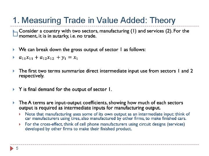
1. Measuring Trade in Value Added: Theory � 5

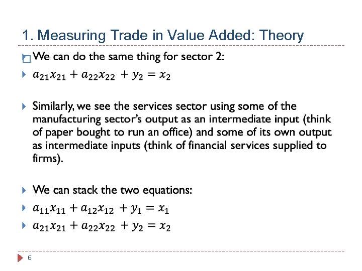
1. Measuring Trade in Value Added: Theory � 6

1. Measuring Trade in Value Added: Theory � 7

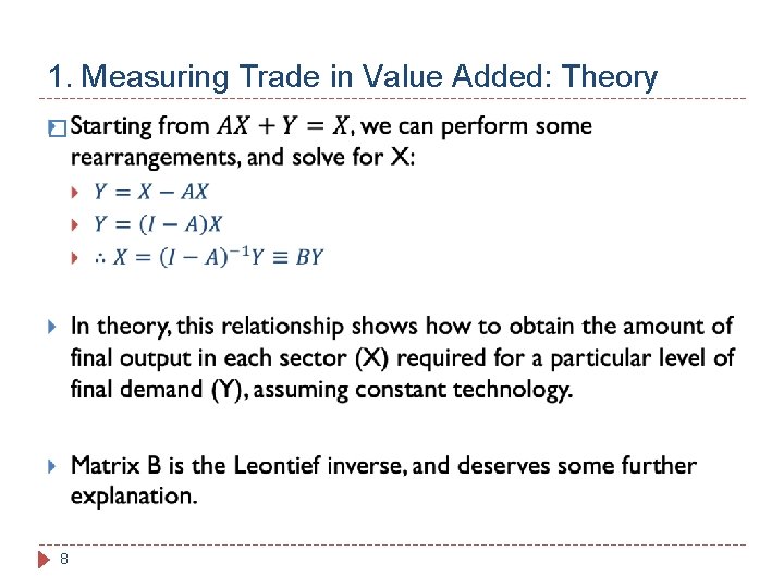
1. Measuring Trade in Value Added: Theory � 8

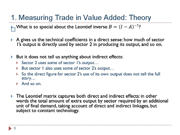
1. Measuring Trade in Value Added: Theory � 9

1. Measuring Trade in Value Added: Theory � 10

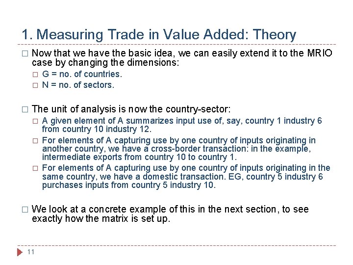
1. Measuring Trade in Value Added: Theory � Now that we have the basic idea, we can easily extend it to the MRIO case by changing the dimensions: � � � The unit of analysis is now the country-sector: � � G = no. of countries. N = no. of sectors. A given element of A summarizes input use of, say, country 1 industry 6 from country 10 industry 12. For elements of A capturing use by one country of inputs originating in another country, we have a cross-border transaction: in the example, intermediate exports from country 10 to country 1. For elements of A capturing use by one country of inputs originating in the same country, we have a domestic transaction. EG, country 5 industry 6 purchases inputs from country 5 industry 10. We look at a concrete example of this in the next section, to see exactly how the matrix is set up. 11

1. Measuring Trade in Value Added: Theory � 12

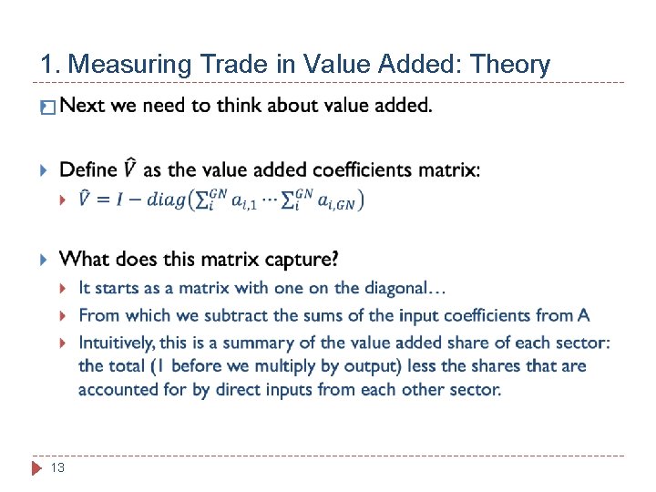
1. Measuring Trade in Value Added: Theory � 13

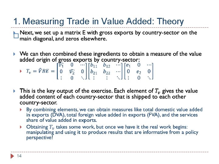
1. Measuring Trade in Value Added: Theory � 14

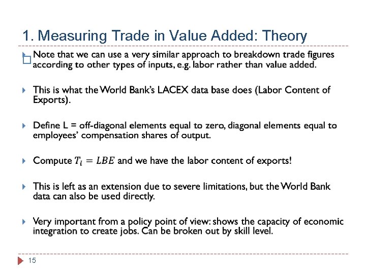
1. Measuring Trade in Value Added: Theory � 15

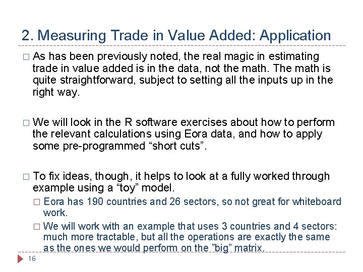
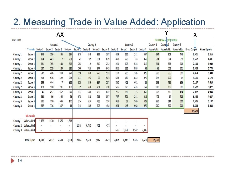
2. Measuring Trade in Value Added: Application � As has been previously noted, the real magic in estimating trade in value added is in the data, not the math. The math is quite straightforward, subject to setting all the inputs up in the right way. � We will look in the R software exercises about how to perform the relevant calculations using Eora data, and how to apply some pre-programmed “short cuts”. � To fix ideas, though, it helps to look at a fully worked through example using a “toy” model. Eora has 190 countries and 26 sectors, so not great for whiteboard work. � We will work with an example that uses 3 countries and 4 sectors: much more tractable, but all the operations are exactly the same as the ones we would perform on the ”big” matrix. � 16

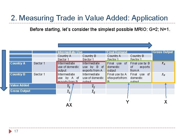
2. Measuring Trade in Value Added: Application Before starting, let’s consider the simplest possible MRIO: G=2; N=1. Country A Sector 1 Country B Sector 1 Intermediate Use Country A Country B Sector 1 Intermediate use of domestic use by B of output exports from A Intermediate use by A of use of domestic exports from B output Final Demand Country A Sector 1 Final use of domestic output Final use by A of exports from B Gross Output Country B Sector 1 Final use by B of exports from A Final use of domestic output Value Added Gross Output AX 17 Y X

2. Measuring Trade in Value Added: Application AX 18 Y X

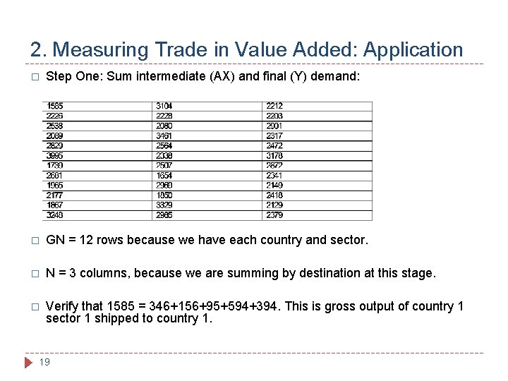
2. Measuring Trade in Value Added: Application � Step One: Sum intermediate (AX) and final (Y) demand: � GN = 12 rows because we have each country and sector. � N = 3 columns, because we are summing by destination at this stage. � Verify that 1585 = 346+156+95+594+394. This is gross output of country 1 sector 1 shipped to country 1. 19

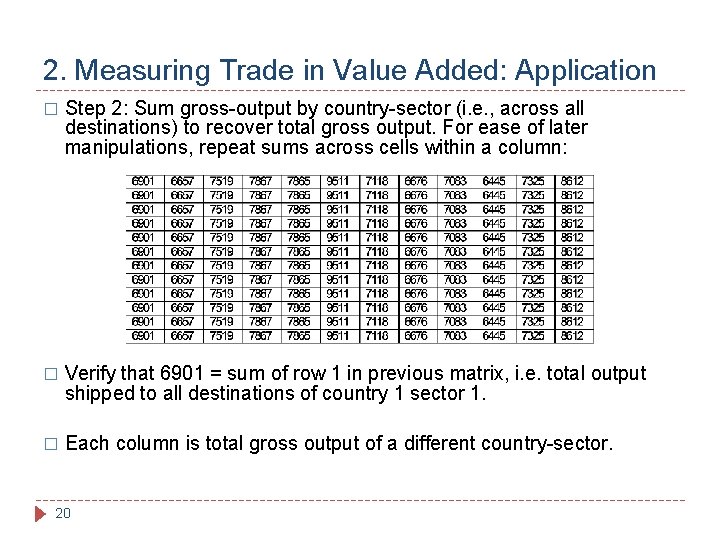
2. Measuring Trade in Value Added: Application � Step 2: Sum gross-output by country-sector (i. e. , across all destinations) to recover total gross output. For ease of later manipulations, repeat sums across cells within a column: � Verify that 6901 = sum of row 1 in previous matrix, i. e. total output shipped to all destinations of country 1 sector 1. � Each column is total gross output of a different country-sector. 20

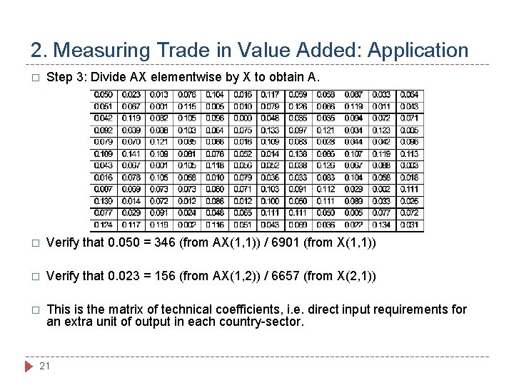
2. Measuring Trade in Value Added: Application � Step 3: Divide AX elementwise by X to obtain A. � Verify that 0. 050 = 346 (from AX(1, 1)) / 6901 (from X(1, 1)) � Verify that 0. 023 = 156 (from AX(1, 2)) / 6657 (from X(2, 1)) � This is the matrix of technical coefficients, i. e. direct input requirements for an extra unit of output in each country-sector. 21

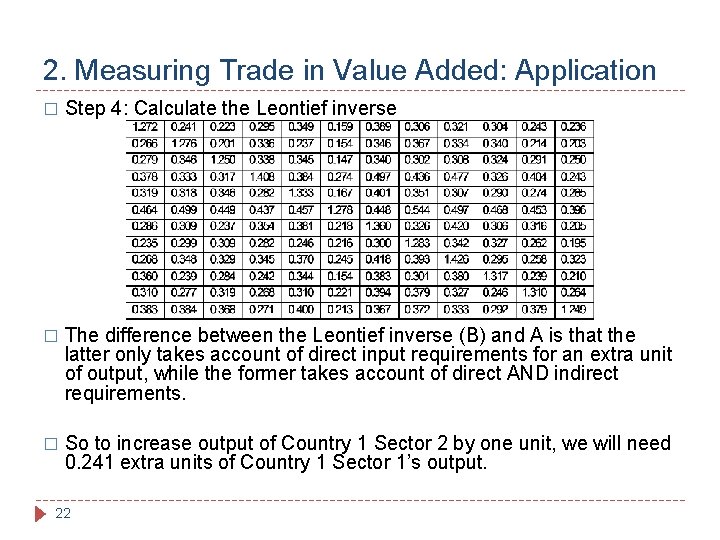
2. Measuring Trade in Value Added: Application � Step 4: Calculate the Leontief inverse � The difference between the Leontief inverse (B) and A is that the latter only takes account of direct input requirements for an extra unit of output, while the former takes account of direct AND indirect requirements. � So to increase output of Country 1 Sector 2 by one unit, we will need 0. 241 extra units of Country 1 Sector 1’s output. 22

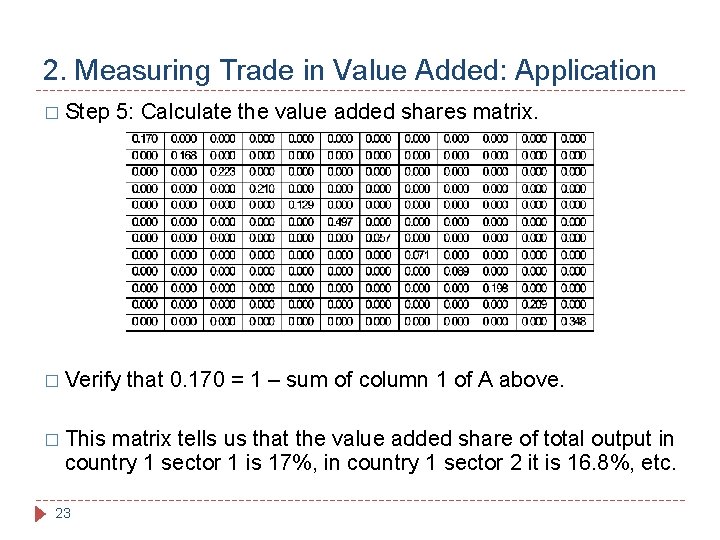
2. Measuring Trade in Value Added: Application � Step 5: Calculate the value added shares matrix. � Verify � This that 0. 170 = 1 – sum of column 1 of A above. matrix tells us that the value added share of total output in country 1 sector 1 is 17%, in country 1 sector 2 it is 16. 8%, etc. 23

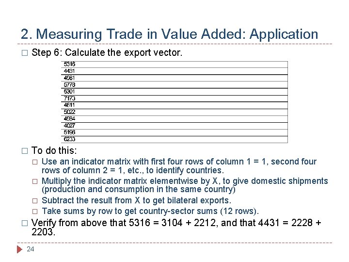
2. Measuring Trade in Value Added: Application � Step 6: Calculate the export vector. � To do this: � � � Use an indicator matrix with first four rows of column 1 = 1, second four rows of column 2 = 1, etc. , to identify countries. Multiply the indicator matrix elementwise by X, to give domestic shipments (production and consumption in the same country) Subtract the result from X to get bilateral exports. Take sums by row to get country-sector sums (12 rows). Verify from above that 5316 = 3104 + 2212, and that 4431 = 2228 + 2203. 24

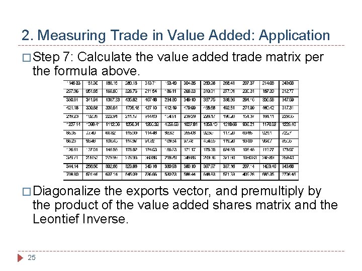
2. Measuring Trade in Value Added: Application � Step 7: Calculate the value added trade matrix per the formula above. � Diagonalize the exports vector, and premultiply by the product of the value added shares matrix and the Leontief Inverse. 25

2. Measuring Trade in Value Added: Application � The R statistics package makes it easy for us to do this work. � See the sample code provided for a detailed explanation. � Use the Decompr package to obtain: The Leontief decomposition, as above, but in list rather than matrix form. � The WWZ decomposition, discussed below. � � For understanding the nature of the analysis, the Leontief decomposition is very helpful. But for interpretation and quantitative work, the WWZ decomposition is frequently more helpful. 26

3. Making the Data “Talk” � Making the data “talk” is not about torturing them until they say what we want! � Rather, the objective is to use simple approaches to take sophisticated output and make it policy-relevant and easily understandable. � One way of doing that is to start with the Tv matrix calculated previously, but then work to produce interesting aggregates. � Obtaining Tv from raw data really needs a matrix algebra engine or statistics package (R, Matlab, Octave, Stata, SAS, SPSS, etc. ). Excel does not make it it easy to do matrix algebra with large matrices. � But once we have Tv, we can use Excel to produce the aggregates we are interested in. � 27 Or those comfortable in one of the packages above can easily continue in it.

3. Making the Data “Talk” � An alternative used by many researchers is the WWZ decomposition (Wang et al. , 2013). � It takes an accounting approach to decomposing gross exports into their value added components. � Output from WWZ produces the following quantities: Domestic value added in final exports (DVA_FIN). � Domestic value added in intermediate exports (DVA_Int, DVA_INTrex. I 1, DVA_INTrex. F, DVA_INTrex. I 2). � Domestic value added returning home (RDV_INT, RDV_FIN 2). � Foreign value added in exports (FVA = MVA_FIN + OVA_FIN + MVA_INT + OVA_INT). � Pure double counting (PDC = DDC + ODC + MDC). � 28

3. Making the Data “Talk” � Output from the WWZ decomposition can be used directly to calculate quantities of interest for GVC analysis: � Gross Exports = Sum(All elements) � FVA = MVA_FIN + OVA_FIN + MVA_INT. � DVA = Gross Exports – FVA. � Backward linkages = FVA / Gross Exports. � DVX = RDV_INT + RDV_FIN 2 + DDC_FIN + DDC_INT + DVA_INTrex. I 1 + DVA_INTrexf + DVA_INTrex. I 2. � Forward linkages = DVX / Gross Exports. � GVC participation = Backward Linkages + Forward Linkages. 29

3. Making the Data “Talk” � Aggregating relevant: in this way can help provide results that are policy DVA and FVA shares over time. � GVC participation index over time. � Services DVA and FVA shares over time, as an indicator of the degree of servicification of value chains in different sectors and countries. � � For those with a background in math and statistics, packages like R can be used to automate the aggregation process to produce useful results by country or by sector. � For others, once we have Tv or the WWZ decomposition, we can shift to working in Excel: it’s more laborious, but if we’re clear on the intuition and the interpretation, we can easily compute interesting figures this way. 30

Key Takeaways 1. Calculating trade in value added requires a lot of data and hard work, and a little math. 2. The basic ingredients are trade data and IO tables, which are then linked together to produce a harmonized MRIO. 3. The algebra involves basic input-output relations and the Leontief inverse, which have been well understood since the 1950 s but only recently applied to trade. 4. Working with a “toy” model helps fix ideas and get the intuition straight, before moving to real data. 5. Knowledge of a statistical package is necessary to produce the full matrix of value added by origin, but once this is available, aggregate results can in theory be produced using Excel (with a bit of work and willingness to manipulate 20, 000 data points). 6. UNCTAD has produced helpful indicators using Eora for 190 countries, which participants should be familiar with. But to look at services RVCs and GVCs specifically, more detail is required: so we will learn how to calculate the full matrix and work up from there. 31

Additional Resources � Data: � Eora raw data: http: //worldmrio. org. Sign up for a trial account! � UNCTAD Eora GVC indicators: http: //worldmrio. com/unctadgvc/. � Reading: � Bastiaan Quast and Victor Kummritz (2015) “decompr: Global Value Chain Decomposition in R”, https: //bit. ly/2 RZkx. UR. � Aqib Aslam et al. (2017) “Calculating Trade in Value Added. ” (IMF), https: //bit. ly/2 QTCCDO. � Zhi Wang et al. (2013) “Quantifying International 32 Production Sharing at the Bilateral and Sector Levels”,