Jody Culham Brain and Mind Institute Department of

Jody Culham Brain and Mind Institute Department of Psychology Western University http: //www. fmri 4 newbies. com/ f. MRI Analysis with emphasis on the General Linear Model Last Update: October 24, 2016 Last Course: Psychology 9223, F 2016, Western University

From Design to Data

The GLM for Math Whizzes Friston 2005, Ann. Rev. Psych.

The GLM visually/intuitively when 1=2 = + + when 2=0. 5 f. MRI Signal “our data” = = Design Matrix x Betas “what we CAN explain” x “how much of it we CAN explain” + Residuals + “what we CANNOT explain” Statistical significance is basically a ratio of explained to unexplained variance
 TR = 2")
Simple Two-Condition Paradigm Visual Stimuli Baseline (blank screen with fixation point) TR = 2 s/volume Duration = 8 min, 44 s = 524 s #Volumes = 262

Let’s Start with One Voxel in Occipital Cortex
 Time (2 -s volumes)")
One Occipital Voxel’s Time Course Activation (Raw) Time (2 -s volumes)
 Time (2 -s volumes)")
Voxel Compared to Protocol Activation (Raw) Time (2 -s volumes)
 Time (2 -s volumes) % BOLD Signal Change")
Y-Axis Converted to %BSC Activation (Raw) Time (2 -s volumes) % BOLD Signal Change for each timepoint Y%BSC = (Yraw – Ybaseline)/Ybaseline)

Linear Correlation

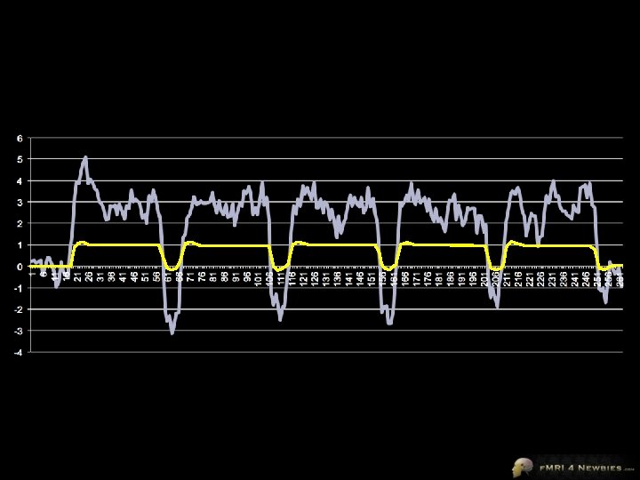
%BSC 0. 23 0. 28 0. 17 0. 23 0. 30 -0. 39 -0. 05 0. 39 0. 42 0. 09 -0. 29 -0. 96 -0. 75 0. 21 -0. 23 -0. 39 -0. 53 0. 61 1. 52 3. 23 3. 89 3. 86 4. 51 4. 82 5. 08 3. 85 Square. Wave … 0 0 0 0 1 1 1 Correlation Between Square-Wave Predictor and Time Course Data r 0. 59872977 r^2 0. 358477338 data points 262 df 260

Correlation Between %BSC and SW Predictor

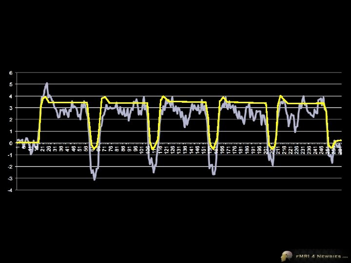
How Can We Do Better? Use HRF We can convolve our square wave predictor with an HRF model Note: we can choose which HRF model to use

Correlation Between %BSC and HRF Predictor

Correlation Between %BSC and HRF Predictor

Just a few more times • There are 60, 199 voxels in this data set • So we just have to do this 60, 198 more times…

Effect of Minimum Thresholds r =. 80 64% of variance p < ran out of digits r =. 60 36% of variance p < 10 -26 Maximum Threshold Cosmetic r =. 40 16% of variance p < 10 -10 r >=. 80 Minimum Threshold Important! positively correlated with predictor (stimulus > baseline) r >. 40 r =. 12 1% of variance p <. 05 r < -. 80 r < -. 40 r=0 0% of variance p <= 1 Maximum Threshold Cosmetic Minimum Threshold Important! negatively correlated with predictor (stimulus < baseline)

Effect of Maximum Thresholds r =. 40 16% of variance p < 10 -10 r >=. 60 r >=. 80 r >= 1 r >. 40 Change maximum threshold to match most significant region so your data span the full range

GLM: 1 predictor

GLM: 1 predictor • Why do we have only one predictor when there are two conditions -- Stimulus and Baseline? • Why not add…

Analogy • How many degrees of freedom are in this equation with two variables? • i. e. , how many things can you change? x+y=7

0 -1 -2 -3 -4 1 6 11 16 21 26 31 36 41 46 51 56 61 66 71 76 81 86 91 96 101 106 111 116 121 126 131 136 141 146 151 156 161 166 171 176 181 186 191 196 201 206 211 216 221 226 231 236 241 246 251 256 261 6 5 4 3 2 1

We have 1 degree of freedom here • Adjust the height of the predictor function to match the data β=1 4 3 2 1 0 -1 -2 -3 -4 -5 β=2 β=4 β=0 β = -1 β = -5

The beta weight is NOT a correlation • correlations measure goodness of fit regardless of scale • beta weights are a measure of scale small ß large r small ß small r large ß large r large ß small r

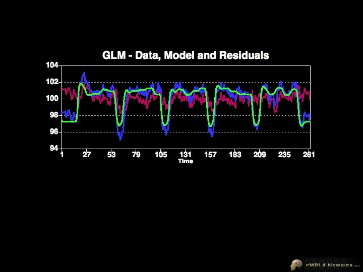
Brain Voyager’s Model
")
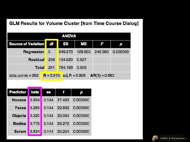
Brain Voyager’s Output Our model had only 1 df Remaining df is noise (residuals) In a model for a single subject, total df = volumes - 1 Our model accounts for variance of 635 Total variance = 784 Our model accounts for R 2 = 0. 92 = 81% of the variance 635/784 = 81%

Brain Voyager’s Output F test F = MSsignal/Msnoise F = 635/0. 576 = 1102 Look up F of 1102 with df =260 p <. 000001 MS = SS/df

Brain Voyager’s Output Look up t = 33. 2 with 260 df p<. 000001 se is an estimate of noise for our beta Remember our 1 df (height of predictor) This is it – our β t = signal/noise = β/se = 3. 591/0. 108 = 33. 2

Comparison Correlation GLM • both maps set to p <. 00001 with 260 df • correlation yields r map (r<. 27) • GLM yields t map (t>4. 51)
 GLM definition from Huettel et al. : • a")
The General Linear Model (GLM) GLM definition from Huettel et al. : • a class of statistical tests that assume that the experimental data are composed of the linear combination of different model factors, along with uncorrelated noise • Model – statistical model • Linear – things add up sensibly (1+1 = 2) • note that linearity refers to the predictors in the model and not necessarily the BOLD signal • General – many simpler statistical procedures such as correlations, t-tests and ANOVAs are subsumed by the GLM

A More Complex Design • Actually, we had more conditions • There were multiple categories of visual stimuli Houses Faces Objects Bodies Scrambled Images

Now we have 5 df • Now we have 5 degrees of freedom Houses Faces Objects Bodies Scrambled Images Each predictor goes from 0 to 1 We can estimate the amount of activation for each condition by looking at how much we have to scale the predictor to best fit the data
")
Let’s look at another voxel (in PPA)

Our Second Voxel’s Data
 for Houses than")
Our Second Voxel’s Model This voxel shows sig higher activity (β) for Houses than baseline … but NOT sig higher activity (β) for Faces than baseline

But are Houses Sig > than other stims? 1 x βHouses -1 x βFaces 0 x βObjects 0 x βBodies 0 x βScrambled Images i. e. , βHouses - βFaces Contrast Vectors a vector is just a row (or column) of numbers

But are Houses > Faces? 1 -1 0 0 0 Houses – Faces βHouses – βFaces = 1. 031 – 0. 147 = 0. 884

Is this Difference Significant? se = noise estimate for contrast t = signal/noise =0. 884/0. 109 = 8. 075 Look up t (df=260) = 8. 075 p <. 000001

Simple Example Experiment: LO Localizer Lateral Occipital Complex • responds when subject views objects Intact Objects Blank Screen TIME (Unit: Volumes) One volume (12 slices) every 2 seconds for 272 seconds (4 minutes, 32 seconds) Condition changes every 16 seconds (8 volumes) Scrambled Objects

If you only pay attention to one slide in this lecture, it should be the next one!!!

Example: GLM with 2 predictors × 1 = + + × 2 f. MRI Signal “our data” = = Design Matrix x Betas “what we CAN explain” x “how much of it we CAN explain” + Residuals + “what we CANNOT explain” Statistical significance is basically a ratio of explained to unexplained variance

Implementation of GLM in SPM Time Many thanks to Øystein Bech Gadmar for creating this figure in SPM Intact Predictor • • • Scrambled Predictor SPM represents time as going down SPM represents predictors within the design matrix as grayscale plots (where black = low, white = high) over time GLM includes a constant to take care of the average activation level throughout each run – SPM shows this explicity (BV may not)

We create a GLM with 2 predictors when 1=2 = + + when 2=0. 5 f. MRI Signal “our data” = = Design Matrix x Betas “what we CAN explain” x “how much of it we CAN explain” + Residuals + “what we CANNOT explain” Statistical significance is basically a ratio of explained to unexplained variance

How to Reduce Noise • If you can’t get rid of an artifact, you can include it as a “predictor of no interest” to soak up variance Example: Some people include predictors from the outcome of motion correction algorithms Corollary: Never leave out predictors for conditions that will affect your data (e. g. , error trials) This works best when the motion is uncorrelated with your paradigm (predictors of interest)

Including First Derivative • Some recommend including the first derivative of the HRF-convolved predictor – can soak up some of the variance due to misestimations of the HRF

Now do you understand why we did temporal filtering? raw data highpass lowpass bandpass Poldrack, Mumford & Nichols, 2011 f. MRI Data Analysis

Common Predictors of No Interest • People often include these to reduce residuals – motion parameters – signal from ventricles – models for error trials

Contrasts: Examples with Real Data

Sam’s Paradigm: Localizer for Ventral-Stream Visual Areas Fusiform Face Area

Contrasts in the GLM • We can examine whether a single predictor is significant (compared to the baseline) R L z = -20 • We can also examine whether a single predictor is significantly greater than another predictor

Contrast Vectors Houses Faces Objects Bodies Scram Faces - Baseline 0 +1 0 0 0 Faces - Houses -1 +1 0 0 0 Faces - Objects 0 +1 -1 0 0 Faces - Bodies 0 +1 0 -1 0 Faces - Scrambled 0 +1 0 0 -1

Balanced Contrasts β 1 2 1 1 1 Condition Unbalanced Balanced Contrast -1 +1 -1 -1 -1 β 1 2 1 1 1 Contrast xβ -1 2 -1 -1 -1 Σ=-3 Σ=-2 If you do not balance the contrast, you are comparing one condition vs. the sum of all the others Contrast -1 +4 -1 -1 -1 β 1 2 1 1 1 Contrast xβ -1 8 -1 -1 -1 Σ=-0 Σ=4 If you balance the contrast, you are comparing one condition vs. the average of all the others

Problems with Bulk Contrasts β β 1 2 1 1 1 2 Condition 2 2 2. 5 Condition Balanced: Faces vs. Other Contrast -1 +4 -1 -1 -1 β 1 2 1 1 1 Contrast xβ -1 8 -1 -1 -1 Balanced: Faces vs. Other Σ=0 Σ=4 Contrast -1 +4 -1 -1 -1 β 2 2 0. 5 Contrast xβ -2 8 -2 -2 -0. 5 Σ=1. 5 • Bulk contrasts can be significant if only a subset of conditions differ Σ=0
 Houses Faces Objects Bodies Scram Faces - Baseline 0 +1")
Conjunctions (sometimes called Masking) Houses Faces Objects Bodies Scram Faces - Baseline 0 +1 0 0 0 Faces - Houses -1 +1 0 0 0 Faces - Objects 0 +1 -1 0 0 Faces - Bodies Faces - Scrambled 0 0 +1 +1 0 0 -1 AND AND To describe this in text: • [(Faces > Baseline) AND (Faces > Houses) AND (Faces > Objects) AND (Faces > Bodies) AND (Faces > Scrambled)]

Conjunction Example Faces – Houses Faces – Objects Faces – Bodies Superimposed Maps Faces – Scrambled Faces – Baseline Conjunction

P Values for Conjunctions • If the contrasts are independent: • e. g. , [(Faces > Houses) AND (Scrambled > Baseline)] – pcombined = (psinglecontrast)numberofcontrasts • e. g. , pcombined = (0. 05)2 = 0. 0025 • If the contrasts are non-independent: • e. g. , [(Faces > Houses) AND (Faces > Baseline)] – pcombined is less straightforward to compute

Dealing with Faulty Assumptions

What’s this #*%&ing reviewer complaining about? ! 1. Correction for multiple comparisons 2. Correction for serial correlations – – only necessary for data from single subjects not necessary for group data

Types of Errors Is the region truly active? Yes No Does our stat test indicate that the region is active? Yes HIT Type II Error No Type I Error Correct Rejection Slide modified from Duke course p value: probability of a Type I error e. g. , p <. 05 “There is less than a 5% probability that a voxel our stats have declared as “active” is in reality NOT active

Dead Salmon poster at Human Brain Mapping conference, 2009 • 130, 000 voxels • no correction for multiple comparisons

Fishy Headlines

Mega-Multiple Comparisons Problem Typical 3 T Data Set 30 slices x 64 = 122, 880 voxels of (3 mm)3 If we choose p < 0. 05… 122, 880 voxels x 0. 05 = approx. 6144 voxels should be significant due to chance alone We can reduce this number by only examining voxels inside the brain ~64, 000 voxels (of (3 mm)3) x 0. 05 = 3200 voxels significant by chance
 –")
Possible Solutions to Multiple Comparisons Problem • Bonferroni Correction (Family-wise Error, FWE Correction) – small volume correction • • Cluster Correction Gaussian Random Field Theory False Discovery Rate Test-Retest Reliability
 Correction • divide desired p value by number of comparisons Example: desired")
Bonferroni (FWE) Correction • divide desired p value by number of comparisons Example: desired p value: p <. 05 number of voxels in brain: 64, 000 required p value: p <. 05 / 64, 000 p <. 00000078 • Variant: small-volume correction • only search within a limited space • brain • cortical surface • region of interest • reduces the number of voxels and thus the severity of Bonferroni • Drawback: overly conservative • assumes that each voxel is independent of others • not true – adjacent voxels are more likely to be sig in f. MRI data than non-adjacent voxels

Cluster Correction • • • falsely activated voxels should be randomly dispersed set minimum cluster size (k) to be large enough to make it unlikely that a cluster of that size would occur by chance some algorithms assume that data from adjacent voxels are uncorrelated (not true) some algorithms (e. g. , Brain Voyager) estimate and factor in spatial smoothness of maps • cluster threshold may differ for different contrasts Drawbacks: • handicaps small regions (e. g. , subcortical foci) more than large regions • researcher can test many combinations of p values and k values and publish the one that looks the best
 Step")
How cluster correction works • • Step 1: Choose a cluster-defining threshold (CDT) Step 2: Estimate smoothness of maps Step 3: Run Monte Carlo simulations on randomly generated maps with the smoothness determined in Step 2 to determine the likelihood of finding clusters of different sizes Step 4: Set a minimum cluster size (k) and exclude any clusters of voxels that are smaller

Gaussian Random Field Theory • • Fundamental to SPM If data are very smooth, then the chance of noise points passing threshold is reduced Can correct for the number of “resolvable elements” (“resels”) rather than number of voxels Drawback: Requires smoothing Slide modified from Duke course

False Discovery Rate • • “controls the proportion of rejected hypotheses that are falsely rejected” (Type II errors) standard p value (e. g. , p <. 01) means that a certain proportion of all voxels will be significant by chance (1%) FDR uses q value (e. g. , q <. 01), meaning that a certain proportion of the “activated” (colored) voxels will be significant by chance (1%) Drawbacks • very conservative when there is little activation; less conservative when there is a lot of activation

Test-Retest Reliability • • Perform statistical tests on each half of the data The probability of a given voxel appearing in both purely by chance is the square of the p value used in each half e. g. , . 001 x. 001 =. 000001 Alternatively, use the first half to select an ROI and the second half to test your hypothesis Drawback: By splitting your data in half, you’re reducing your statistical power to see effects

Strategies for Publication vs Piloting • Publication – Have a specific hypothesis/contrast planned – Run all your subjects – Run the stats as planned with all necessary corrections – Publish • Piloting – Run a few subjects to see if you’re on the right track – Spend a lot of time exploring the pilot data for interesting patterns – “Find the story” in the data – You may even change the experiment, run additional subjects, or run a follow-up experiment to chase the story • While you need to use rigorous corrections for publication, do not be overly conservative when exploring pilot data or you might miss interesting trends • Random effects analyses can be quite conservative so you may want to do exploratory analyses with fixed effects (and then run more subjects if needed so you can publish random effects)

Sanity Checks: “Poor Man’s Bonferroni” • • • For casual data exploration, not publication Jack up the threshold till you get rid of the schmutz (especially in air, ventricles, white matter – may be real) If you have a comparison where one condition is expected to produce much more activity than the other, turn on both tails of the comparison If two areas are symmetrically active, they’re less likely to be due to chance (only works for bilateral areas) Jody’s rule of thumb: “If ya can’t trust the negatives, can ya trust the positives? ” Too subjective for serious use Example: MT+ localizer data Moving rings > stationary rings (orange) Stationary rings > moving rings (blue)

Have We Been So Obsessed with Limiting Type I Error that Type II Error is Out of Control? Yes No Yes HIT Type I Error No Does our stat test indicate that the region is active? Is the region truly active? Type II Error Correct Rejection Slide modified from Duke course

Comparison of Methods simulated data uncorrected -high Type I -low Type II Bonferroni -low Type I -high Type II FDR -low Type II Poldrack, Mumford & Nichols, 2011 f. MRI Data Analysis

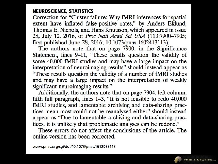
What a Clusterf… ailure! 2016 • resting-state data from Functional Connectomes Project • applied stats to test for task-based “activation” using SPM, FSL and AFNI software packages • since there was no real task-based activation, false positives for cluster correction should be 5% • tested block designs and event-related designs with varying degrees of spatial smoothing (4 -, 6 -, 8 -, and 10 -mm FWHM)

p=. 05 EXPECTED What a Clusterf… ailure! p>>>. 05 ACTUAL n=20, FWHM = 6 mm Cluster threshold p<. 01 2016 n=20 , FWHM = 6 mm Cluster threshold p<. 001 n=20 , FWHM = 6 mm Voxel

Why So Wrong? • AFNI had a bug for 15 years • Tests assume that spatial correlations have a particular shape (squared exponential distribution) – wrong! • Tests assume constant spatial smoothness across the brain – wrong! Expected shape of spatial correlations does not match actual shape Some areas (esp. posterior cingulate) have higher-than-average smoothness and thus higher false positives

Beware scientific click-bait

The Sky is Falling!

• Not all blobs in all studies are vulnerable to this problem (many blobs sig above thresholds, not every study went fishing for blobs) • False positives weren’t too bad at p<. 001 • Future software can incorporate better approaches such as non-parametric permutation testing (computationally intensive) http: //www. ohbmbrainmappingblog. com/blog/keep-calm-and-scan-on http: //blogs. discovermagazine. com/neuroskeptic/2015/12/07/false-positive-fmri-revisited/#. WA 2 DAZMr. Js. M http: //blogs. discovermagazine. com/neuroskeptic/2016/07/07/false-positive-fmri-mainstream http: //brainvoyager. com/bvresources/Rainers. BVBlog/files/a 8 a 22212 f 9 f 1 f 01 e 4 da 11 fef 4 ba 91 da 8 -34. html

What’s this #*%&ing reviewer complaining about? ! 1. Correction for multiple comparisons 2. Correction for serial correlations – – only necessary for data from single subjects not necessary for group data • stay tuned to find out why: Group Data lecture

Correction for Temporal Correlations When analyzing a single subject, degrees of freedom = number of volumes – 1 e. g. , if our run has 200 volumes (400 s long if TR = 2), then df = 199 Statistical methods assume that each of our time points is independent. In the case of f. MRI, this assumption is false. Even in a “screen saver scan”, activation in a voxel at one time is correlated with it’s activation within ~6 sec This artificially inflates your statistical significance.

Autocorrelation function original To calculate the magnitude of the problem, we can compute the autocorrelation function on the residuals shift by 1 volume For a voxel or ROI, correlate its time course with itself shifted in time shift by 2 volumes time If there’s no autocorrelation, function should drop from 1 to 0 abruptly – pink line The points circled in yellow suggest there is some autocorrelation, especially at a shift of 1, called AR(1) Plot these correlations by the degree of shift
 p values BEFORE")
BV can correct for the autocorrelation to yield revised (usually lower) p values BEFORE AFTER

BV Preprocessing Options

Temporal Smoothing of Data • We have the option in our software to temporally smooth our data (i. e. , remove high temporal frequencies or “low-pass filter”) • However, I recommended that you not use this option • Now do you understand why?

To Localize or Not to Localise?

Hypothetical Example • The extrastriate body area responds more to human bodies than to other categories of visual stimuli (e. g. , human faces, places, objects) • You want to know if the extrastriate body area responds more to animal bodies vs. animal faces

Voxelwise Analysis > • Perform GLM for a particular contrast at every voxel in the brain • If you do see activation in the lateral occipitotemporal cortex, is it really EBA? • If you don’t see activation, maybe your statistical test was too conservative because of the correction for multiple comparisons (e. g. , Type II error)

Region of Interest Analysis • One solution is to define your regions independently • Then you can test your contrast in that region at good ol’ p <. 05

ROIs can be defined by functional and/or anatomical criteria images from O’Reilly et al. , 2012, SCAN Functional ROI Anatomical Functional-Anatomical ROI

Localizer can be built into same run as experimental conditions or can be done separately Step 1: Localize ROI using voxelwise contrasts • Human bodies > human faces • Identify EBA Step 2: Test EBA on contrast of interest • Animal bodies > animal faces • Can use simple p <. 05

ROIs should be defined independently • Maybe what we really want to know is whether the difference between human bodies and faces is greater than the difference between animal bodies and faces Human Animal Face Body

Ideally ROIs should be defined independently One option • put all four conditions into one run • Step 1: Identify EBA by human body > human face • Step 2: Test interaction Human Animal Face Body However, this suffers from the non-independence error

Non-independence Error Let’s say on average, this is what really happens in EBA as a whole (ground truth) Human Animal Face Body

Non-independence Error • But we know that there is also noise in the measurement such that different voxels may have slight differences in effects Human Animal Face Voxel 1 Body Face Body Voxel 2 Face Body Voxel 3 • Based on our selection criteria, we’d be likely to include voxel 1 and 2 in our ROI but not voxel 3 • Thus we may erroneously see a significant interaction based on our selection bias

Independent Runs • Because of the non-independence error, we may want to have a separate independent run Localizer Experimental Run • Benefit: Localizer is now based on data independent from experimental run • Cost: We have some redundancy between the localizer and experimental run

ROI Defined at Group or Individual Level Group Analysis Individual Analysis S 1 S 2 S 3 … • The ability to define subject-specific ROIs is one of the advantages of the ROI approach

To Localize or Not to Localise? Neuroimagers can’t even agree how to SPELL localiser/localizer!

Methodological Fundamentalism The latest review I received…

Pros and Cons: Voxelwise Approach Benefits • Require no prior hypotheses about areas involved • Include entire brain • May identify subregions of known areas that are implicated in a function • Doesn’t require independent data set Drawbacks • Requires conservative corrections for multiple comparisons • vulnerable to Type II errors • Neglects individual differences in brain regions • poor for some types of studies (e. g. , topographic areas) • Can lose spatial resolution with intersubject averaging • Requires speculation about areas involved

Pros and Cons: ROI Approach Benefits • Extraction of ROI data can be subjected to simple stats • Elimination of multiple comparisons problem greatly improves statistical power (e. g. , p <. 05) • Hypothesis-driven • Useful when hypotheses are motivated by other techniques (e. g. , electrophysiology) in specific brain regions • ROI is not smeared due to intersubject averaging • Important for discriminating abutting areas (e. g. , V 1/V 2) • Can be useful for dissecting factorial design data in an unbiased manner Drawbacks • Neglects other areas that may play a fundamental role • If multiple ROIs need to be considered, you can spend a lot of scan time collecting localizer data (thus limiting the time available for experimental runs) • Works best for reliable and robust areas with unambiguous definitions • Sometimes you can’t find an ROI in some subjects • Selection of ROIs can be highly subjective and error-prone

ROI and Voxelwise Analyses are NOT mutually exclusive • You can decide based on the situation/hypotheses • You can do both ROI analyses and voxelwise analyses – ROI analyses for well-defined key regions – Voxelwise analyses to see if other regions are also involved • Ideally, the conclusions will not differ • If the conclusions do differ, there may be sensible reasons – Effect in ROI but not voxelwise • perhaps region is highly variable in stereotaxic location between subjects • perhaps voxelwise approach is not statistically powerful enough – Effect in voxelwise but not ROI • perhaps ROI is not homogenous or is context-specific

The War of Non-Independence
4 = 1/28,")
Finding the Obvious A priori probability of getting JQKA sequence = (1/13)4 = 1/28, 561 A posteriori probability of getting JQKA sequence = 1/1 = 100% Non-independence error • occurs when statistical tests performed are not independent from the means used to select the brain region Arguments from Vul & Kanwisher, book chapter in press

Non-independence Error Egregious example • Identify Area X with contrast of A > B • Do post hoc stats showing that A is statistically higher than B • Act surprised!!! More subtle example of selection bias • Identify Area X with contrast of A > B • Do post hoc stats showing that A is statistically higher than C and C is statistically greater than B Arguments from Vul & Kanwisher, book chapter in press Figure from Kriegeskorte et al. , 2009, Nature Neuroscience

Double Dipping & How to Avoid It • Kriegeskorte et al. , 2009, Nature Neuroscience • surveyed 134 papers in prestiguous journals • 42% showed at least one example of nonindependence error

Correlations Between Individual Subjects’ Brain Activity and Behavioral Measures Sample of Critiqued Papers: Eisenberg, Lieberman & Williams, 2003, Science • measured f. MRI activity during social rejection • correlated self-reported distress with brain activity • found r =. 88 in anterior cingulate cortex, an area implicated in physical pain perception • concluded “rejection hurts” social exclusion > inclusion

“Voodoo Correlations” The original title of the paper was not well-received by reviewers so it was changed even though some people still use the term Voodoo 2009 • reliability of personality and emotion measures: r ~. 7 • reliability of activation in a given voxel: r ~. 7 • highest expected behavior: f. MRI correlation is ~. 74 • so how can we have behavior: f. MRI correlations of r ~. 9? !

“Voodoo Correlations” "Notably, 53% of the surveyed studies selected voxels based on a correlation with the behavioral individual-differences measure and then used those same data to compute a correlation within that subset of voxels. " Vul et al. , 2009, Perspectives on Psychological Science

Avoiding “Voodoo” • Use independent means to select region and then evaluate correlation • Do split-half reliability test – WARNING: This is reassuring that the result can be replicated in your sample but does not demonstrate that result generalizes to the population

Is the “voodoo” problem all that bad? • • High correlations can occur in legitimately analyzed data Did voxelwise analyses use appropriate correction for multiple comparisons? – then result is statistically significant regardless of specific correlation • Is additional data being used for 1. – 2. – inference purposes? if they pretend to provide independent support, that’s bad presentation purposes? alternative formats can be useful in demonstrating that data is clean (e. g. , time courses look sensible; correlations are not driven by outliers)
- Slides: 116