Jody Culham Brain and Mind Institute Department of

Jody Culham Brain and Mind Institute Department of Psychology Western University http: //www. fmri 4 newbies. com/ Advanced Designs for f. MRI Last Update: November 17, 2014 Last Course: Psychology 9223, F 2014, Western University

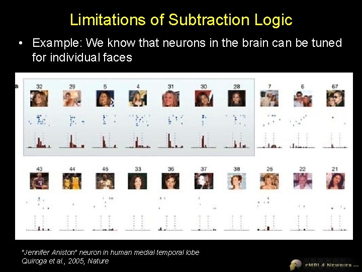
Limitations of Subtraction Logic • Example: We know that neurons in the brain can be tuned for individual faces “Jennifer Aniston” neuron in human medial temporal lobe Quiroga et al. , 2005, Nature

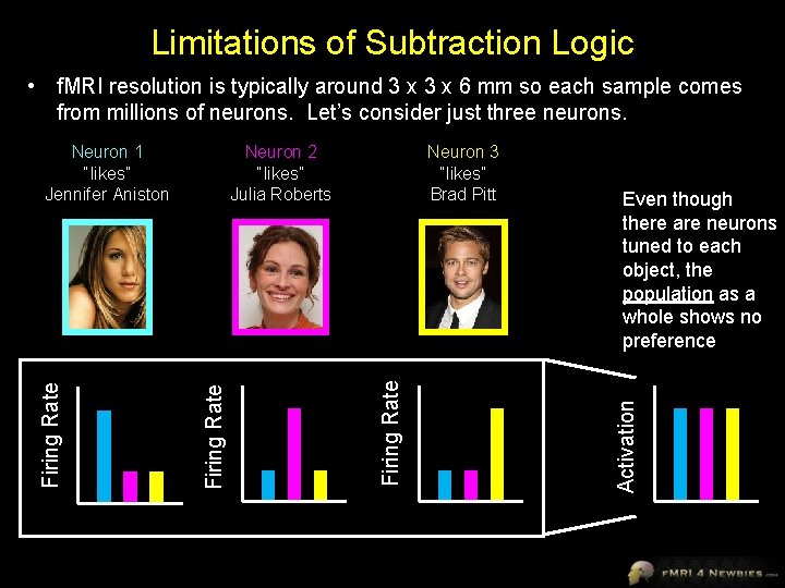
Limitations of Subtraction Logic • f. MRI resolution is typically around 3 x 6 mm so each sample comes from millions of neurons. Let’s consider just three neurons. Even though there are neurons tuned to each object, the population as a whole shows no preference Activation Neuron 3 “likes” Brad Pitt Firing Rate Neuron 2 “likes” Julia Roberts Firing Rate Neuron 1 “likes” Jennifer Aniston

Two Techniques with “Subvoxel Resolution” • “subvoxel resolution” = the ability to investigate coding in neuronal populations smaller than the voxel size being sampled 1. f. MR Adaptation (or repetition suppression or priming) 2. Multivoxel Pattern Analysis (or decoding)

f. MR Adaptation (or repetition suppression or priming…)

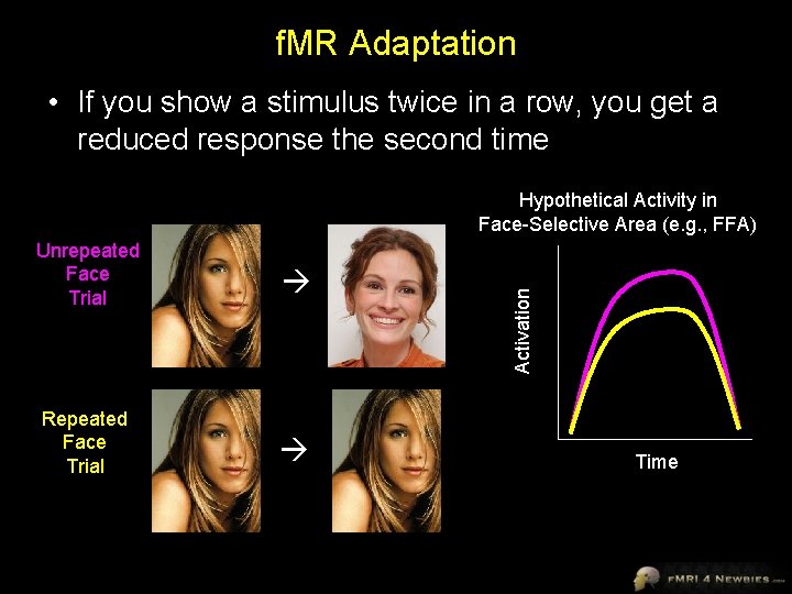
f. MR Adaptation • If you show a stimulus twice in a row, you get a reduced response the second time Unrepeated Face Trial Repeated Face Trial Activation Hypothetical Activity in Face-Selective Area (e. g. , FFA) Time

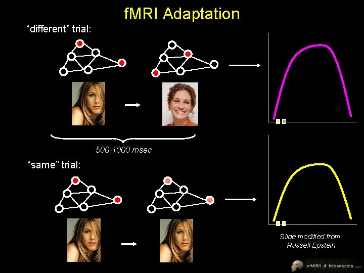
f. MRI Adaptation “different” trial: 500 -1000 msec “same” trial: Slide modified from Russell Epstein

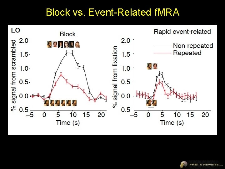
Block vs. Event-Related f. MRA

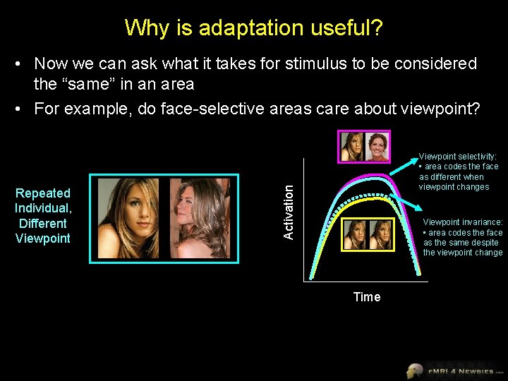
Why is adaptation useful? • Now we can ask what it takes for stimulus to be considered the “same” in an area • For example, do face-selective areas care about viewpoint? Activation Repeated Individual, Different Viewpoint selectivity: • area codes the face as different when viewpoint changes Viewpoint invariance: • area codes the face as the same despite the viewpoint change Time

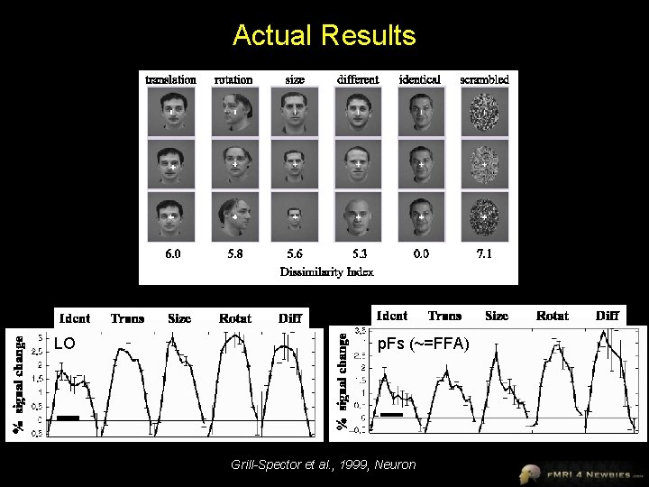
Actual Results LO p. Fs (~=FFA) Grill-Spector et al. , 1999, Neuron

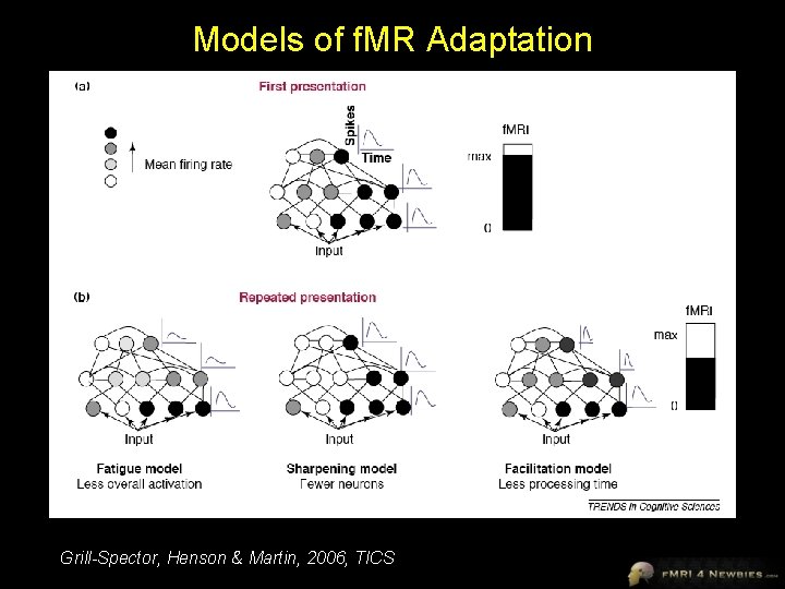
Models of f. MR Adaptation Grill-Spector, Henson & Martin, 2006, TICS

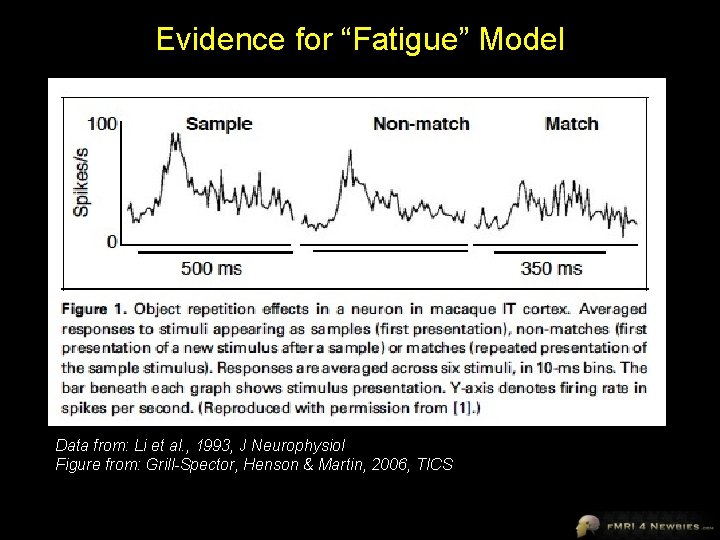
Evidence for “Fatigue” Model Data from: Li et al. , 1993, J Neurophysiol Figure from: Grill-Spector, Henson & Martin, 2006, TICS

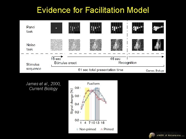
Evidence for Facilitation Model James et al. , 2000, Current Biology

Caveats in Interpreting f. MR Adaptation Results

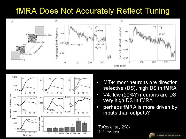
f. MRA Does Not Accurately Reflect Tuning • MT+: most neurons are directionselective (DS), high DS in f. MRA • V 4: few (20%? ) neurons are DS, very high DS in f. MRA • perhaps f. MRA is more driven by inputs than outputs? Tolias et al. , 2001, J. Neurosci

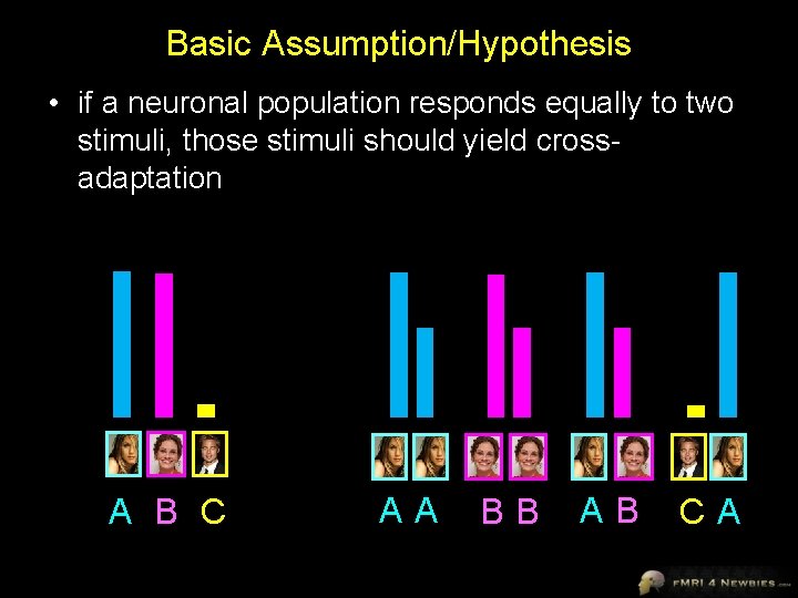
Basic Assumption/Hypothesis Predicted f. MRI Response Neural Response • if a neuronal population responds equally to two stimuli, those stimuli should yield crossadaptation A B C A-A B-B A-B C-A

Experimental Question • the human lateral occipital complex (LOC) is arguably analogous/homologous to macaque inferotemporal (IT) cortex • both human LOC and macaque IT show f. MRI adaptation to repeated objects • Does neurophysiology in macaque IT show object adaptation at the single neuron level?

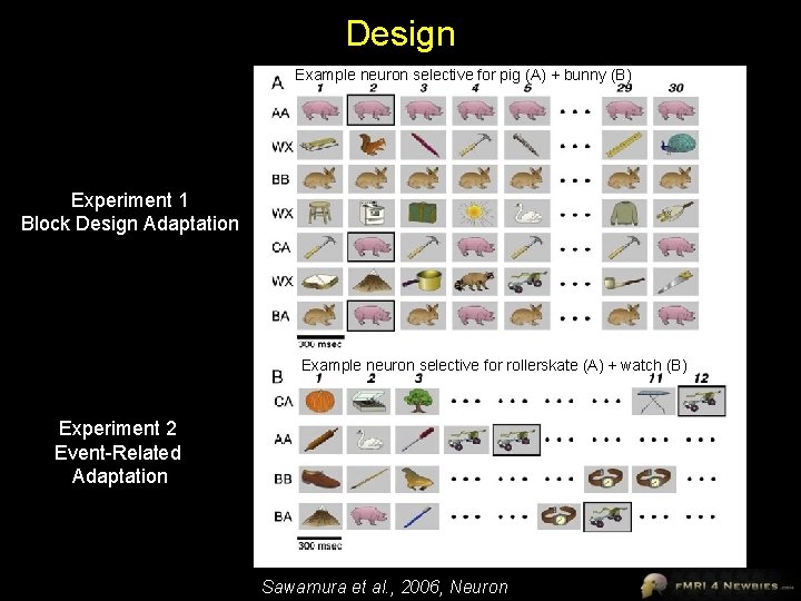
Design Example neuron selective for pig (A) + bunny (B) Experiment 1 Block Design Adaptation Example neuron selective for rollerskate (A) + watch (B) Experiment 2 Event-Related Adaptation Sawamura et al. , 2006, Neuron

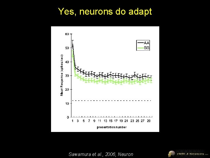
Yes, neurons do adapt Sawamura et al. , 2006, Neuron

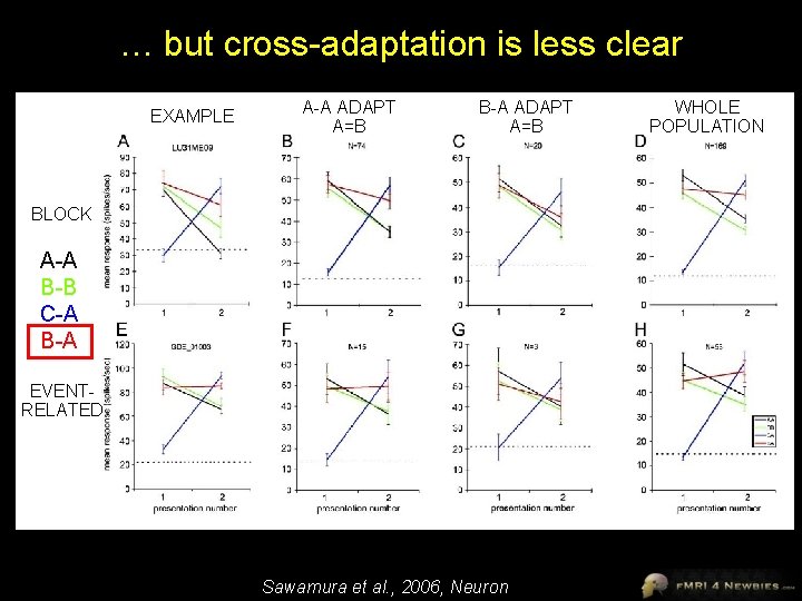
… but cross-adaptation is less clear EXAMPLE A-A ADAPT A=B BLOCK A-A B-B C-A B-A EVENTRELATED Sawamura et al. , 2006, Neuron WHOLE POPULATION

Sawamura et al. Conclusions • Evidence for cross-adaptation at the singleneuron level is not as strong as expected, particularly for event-related designs • They don’t think it’s just attention • Something special about repeated stimuli

Additional Caveats • Adaptation effects are larger when sequence is predictable (Summerfield et al. , 2008, Nat. Neurosci. ) • Adaptation effects can be quite unreliable – variability between labs and studies – even effects that are well-established in neurophysiology and psychophysics don’t always replicate in f. MRA • e. g. , orientation selectivity in primary visual cortex • The effect may also depend on other factors – e. g. , time elapsed from first and second presentation • days, hours, minutes, seconds, milliseconds? • number of intervening items – attention (especially in block designs) – memory encoding • Different areas may demonstrate f. MRA for different reasons – reflected in variety of terms: repetition suppression, priming

So is f. MRA dead? No. Criticism: f. MRA may reflect inputs rather than outputs • Response: This is a general caveat of all f. MRI studies. Inputs are interesting too, just harder to interpret. Focus on outputs oversimplifies neural processing when presumably feedback loops are an essential component. Criticism: f. MRA may not reveal cross-adaptation even in populations that do show cross-coding • Response: This suggests that caution is especially warranted when there is a failure to find cross-adaptation. However, cross-adaptation sometimes does occur. • Note within-item adaptation (A-A or B-B) did occur, so this criticism does not apply in that case.

So is f. MRA dead? No. Criticism: None of the basic models of f. MRA seem to work. • Response: In some ways, it doesn’t matter. The essential use of f. MRA is to determine whether neural populations are sensitive to stimulus dimensions. The exact mechanism for such sensitivity may not be critical. Criticism: f. MRA, and maybe f. MRI in general, is just responding to predictions. • Response: Prediction is interesting too. • Regarding f. MRA, why do some brain areas make predictions about a stimulus while others don’t? • It may be very interesting to figure out how the hemodynamic response can be predictive.

Parametric Designs

Why are parametric designs useful in f. MRI? • As we’ve seen, the assumption of pure insertion in subtraction logic is often false • (A + B) - (B) = A • In parametric designs, the task stays the same while the amount of processing varies; thus, changes to the nature of the task are less of a problem • (A + A) - (A) = A • (A + A) - (A + A) = A

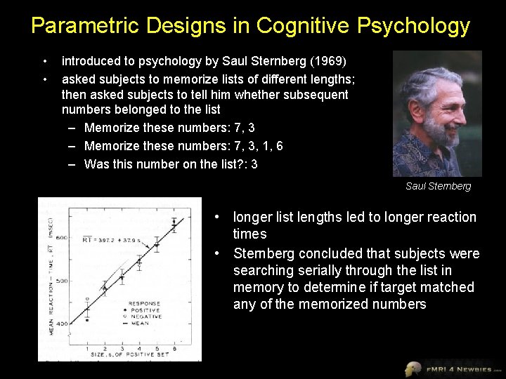
Parametric Designs in Cognitive Psychology • • introduced to psychology by Saul Sternberg (1969) asked subjects to memorize lists of different lengths; then asked subjects to tell him whether subsequent numbers belonged to the list – Memorize these numbers: 7, 3, 1, 6 – Was this number on the list? : 3 Saul Sternberg • longer list lengths led to longer reaction times • Sternberg concluded that subjects were searching serially through the list in memory to determine if target matched any of the memorized numbers

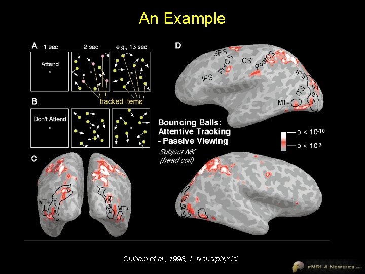
An Example Culham et al. , 1998, J. Neuorphysiol.

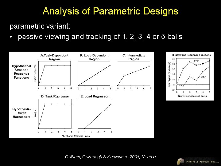
Analysis of Parametric Designs parametric variant: • passive viewing and tracking of 1, 2, 3, 4 or 5 balls Culham, Cavanagh & Kanwisher, 2001, Neuron

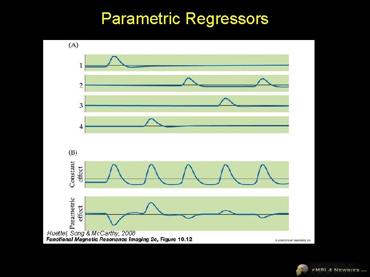
Parametric Regressors Huettel, Song & Mc. Carthy, 2008

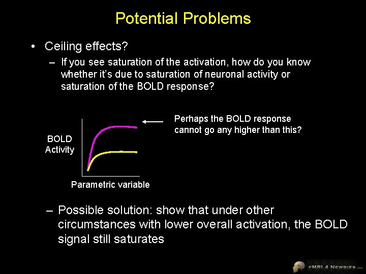
Potential Problems • Ceiling effects? – If you see saturation of the activation, how do you know whether it’s due to saturation of neuronal activity or saturation of the BOLD response? BOLD Activity Perhaps the BOLD response cannot go any higher than this? Parametric variable – Possible solution: show that under other circumstances with lower overall activation, the BOLD signal still saturates

Factorial Designs

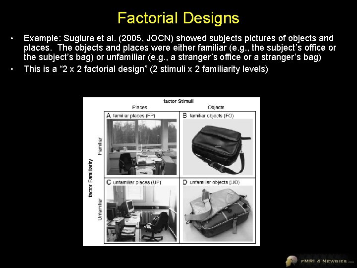
Factorial Designs • • Example: Sugiura et al. (2005, JOCN) showed subjects pictures of objects and places. The objects and places were either familiar (e. g. , the subject’s office or the subject’s bag) or unfamiliar (e. g. , a stranger’s office or a stranger’s bag) This is a “ 2 x 2 factorial design” (2 stimuli x 2 familiarity levels)

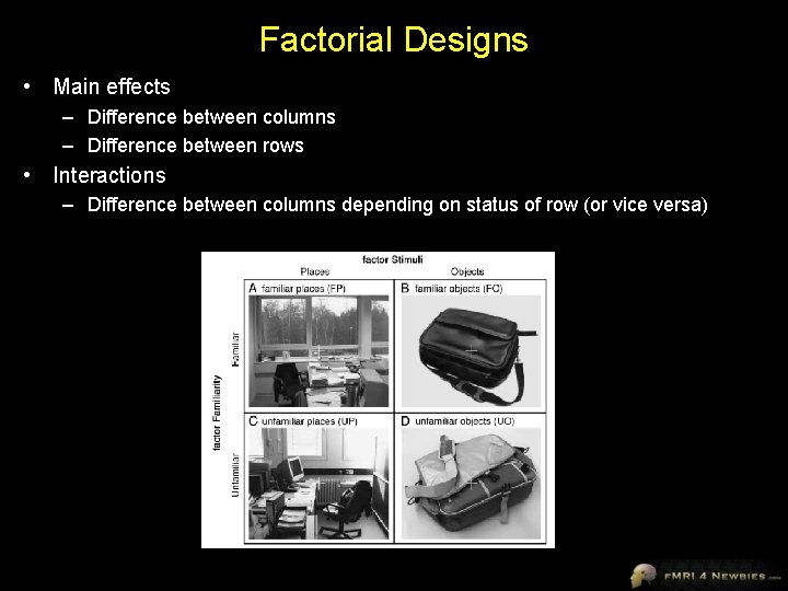
Factorial Designs • Main effects – Difference between columns – Difference between rows • Interactions – Difference between columns depending on status of row (or vice versa)

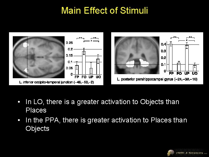
Main Effect of Stimuli • In LO, there is a greater activation to Objects than Places • In the PPA, there is greater activation to Places than Objects

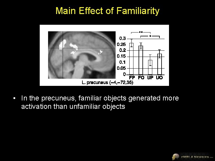
Main Effect of Familiarity • In the precuneus, familiar objects generated more activation than unfamiliar objects

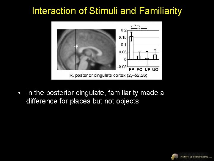
Interaction of Stimuli and Familiarity • In the posterior cingulate, familiarity made a difference for places but not objects

Why do People like Factorial Designs? • If you see a main effect in a factorial design, it is reassuring that the variable has an effect across multiple conditions • Interactions can be enlightening and form the basis for many theories

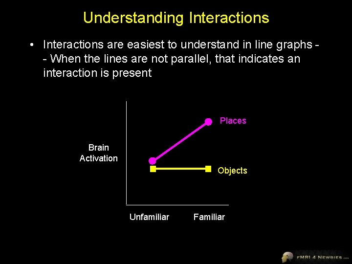
Understanding Interactions • Interactions are easiest to understand in line graphs - When the lines are not parallel, that indicates an interaction is present Places Brain Activation Objects Unfamiliar Familiar

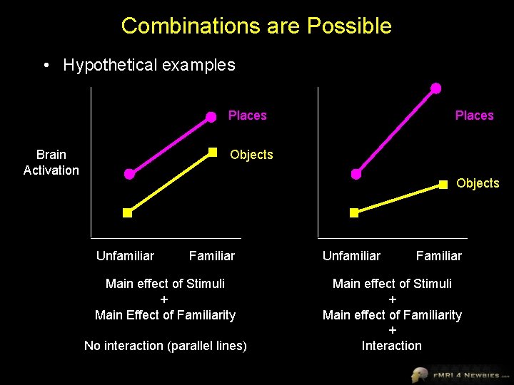
Combinations are Possible • Hypothetical examples Places Brain Activation Places Objects Unfamiliar Familiar Main effect of Stimuli + Main Effect of Familiarity No interaction (parallel lines) Unfamiliar Familiar Main effect of Stimuli + Main effect of Familiarity + Interaction

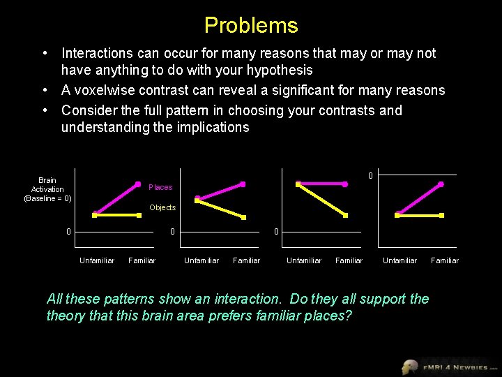
Problems • Interactions can occur for many reasons that may or may not have anything to do with your hypothesis • A voxelwise contrast can reveal a significant for many reasons • Consider the full pattern in choosing your contrasts and understanding the implications 0 Brain Activation (Baseline = 0) Places Objects 0 0 Unfamiliar Familiar Unfamiliar All these patterns show an interaction. Do they all support theory that this brain area prefers familiar places? Familiar

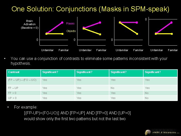
One Solution: Conjunctions (Masks in SPM-speak) 0 Brain Activation (Baseline = 0) Places Objects 0 0 Unfamiliar • Familiar 0 Unfamiliar Familiar Unfamiliar You can use a conjunction of contrasts to eliminate some patterns inconsistent with your hypothesis. Contrast Significant? (FP – UP) – (FO – UO) Yes Yes FP – UP Yes No Yes FP > 0 Yes Yes No UP > 0 Yes Yes No • For example: [(FP-UP)>(FO-UO)] AND [FP>UP] AND [FP>0] AND [UP>0] would show only the first two patterns but not the last two Familiar

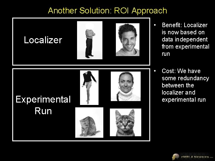
Another Solution: ROI Approach Localizer Experimental Run • Benefit: Localizer is now based on data independent from experimental run • Cost: We have some redundancy between the localizer and experimental run

Problems • Interactions become hard to interpret – one recent psychology study suggests the human brain cannot understand interactions that involve more than three factors • Take home message: Don’t use designs with more than three factors • The more conditions you have, the fewer trials per condition you have Keep it simple!

Group Comparisons: ANOVA

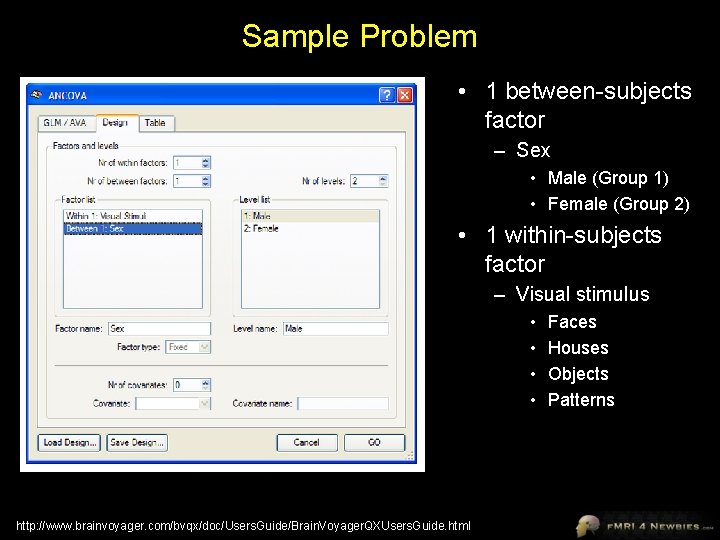
Sample Problem • 1 between-subjects factor – Sex • Male (Group 1) • Female (Group 2) • 1 within-subjects factor – Visual stimulus • • http: //www. brainvoyager. com/bvqx/doc/Users. Guide/Brain. Voyager. QXUsers. Guide. html Faces Houses Objects Patterns

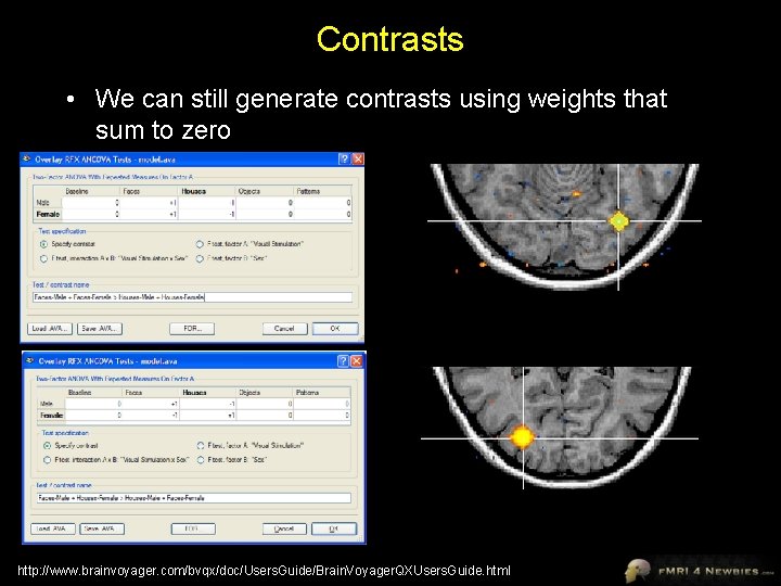
Contrasts • We can still generate contrasts using weights that sum to zero http: //www. brainvoyager. com/bvqx/doc/Users. Guide/Brain. Voyager. QXUsers. Guide. html

Group Comparisons: ANCOVA

ANCOVA Example • Let’s say we have run a face localizer in a group of subjects and want to know if there is a difference in activation between females and males • We may also be concerned about whether age is a confound between groups • We can run an Analysis of Covariance (ANCOVA) to examine the effect of sex differences while controlling for age differences – We say that the effect of age is “partialed out” – This is like pretending that all the subjects were the same age • This reduces the error term for group comparisons, thus increasing statistical power • Between-subjects factor – Sex • Covariate – Age http: //www. brainvoyager. com/bvqx/doc/Users. Guide/Brain. Voyager. QXUsers. Guide. html

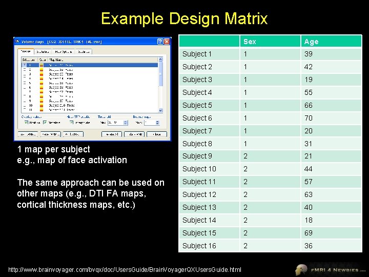
Example Design Matrix 1 map per subject e. g. , map of face activation The same approach can be used on other maps (e. g. , DTI FA maps, cortical thickness maps, etc. ) Sex Age Subject 1 1 39 Subject 2 1 42 Subject 3 1 19 Subject 4 1 55 Subject 5 1 66 Subject 6 1 70 Subject 7 1 20 Subject 8 1 31 Subject 9 2 21 Subject 10 2 44 Subject 11 2 57 Subject 12 2 63 Subject 13 2 40 Subject 14 2 18 Subject 15 2 69 Subject 16 2 36 http: //www. brainvoyager. com/bvqx/doc/Users. Guide/Brain. Voyager. QXUsers. Guide. html

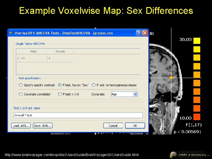
Example Voxelwise Map: Sex Differences http: //www. brainvoyager. com/bvqx/doc/Users. Guide/Brain. Voyager. QXUsers. Guide. html

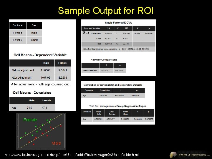
Sample Output for ROI Sex After adjustment = with age covaried out Female Male http: //www. brainvoyager. com/bvqx/doc/Users. Guide/Brain. Voyager. QXUsers. Guide. html

Data-Driven Approaches

Hypothesis- vs. Data-Driven Approaches Hypothesis-driven Examples: t-tests, correlations, general linear model (GLM) • a priori model of activation is suggested • data is checked to see how closely it matches components of the model • most commonly used approach Data-driven Example: Independent Component Analysis (ICA) • blindly separates a set of statistically independent signals from a set of mixed signals • no prior hypotheses are necessary

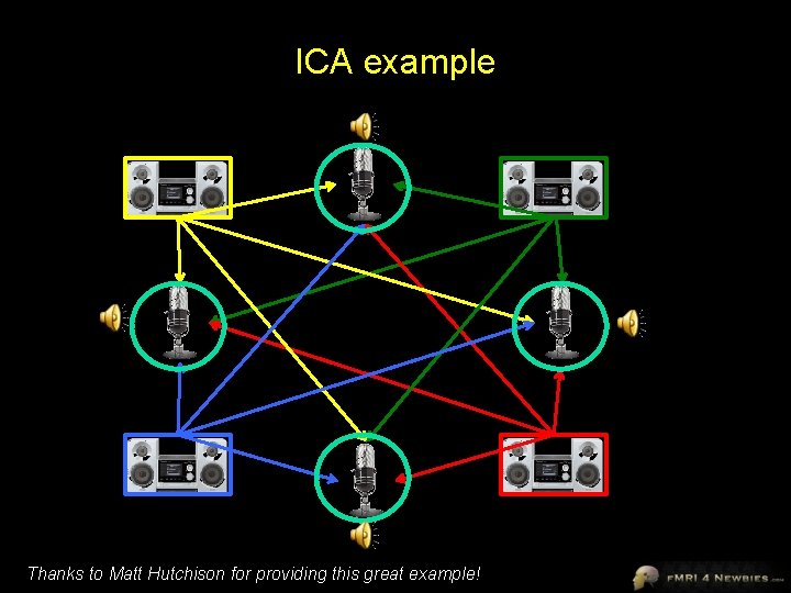
ICA example Thanks to Matt Hutchison for providing this great example!

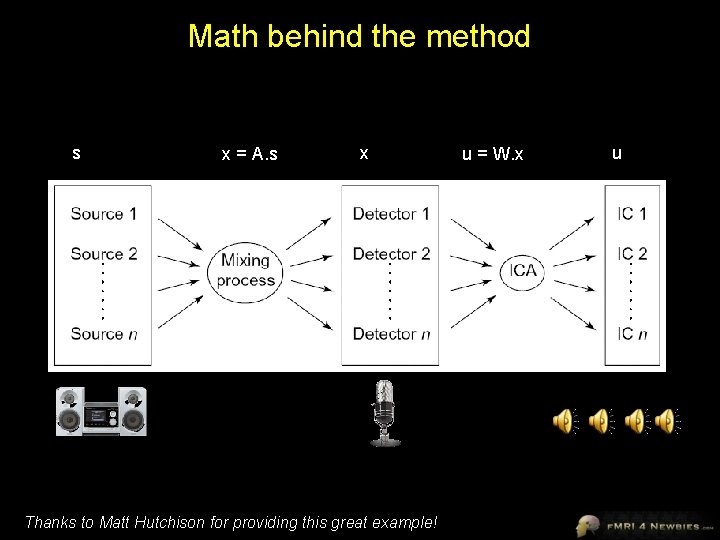
Math behind the method s x = A. s x Thanks to Matt Hutchison for providing this great example! u = W. x u

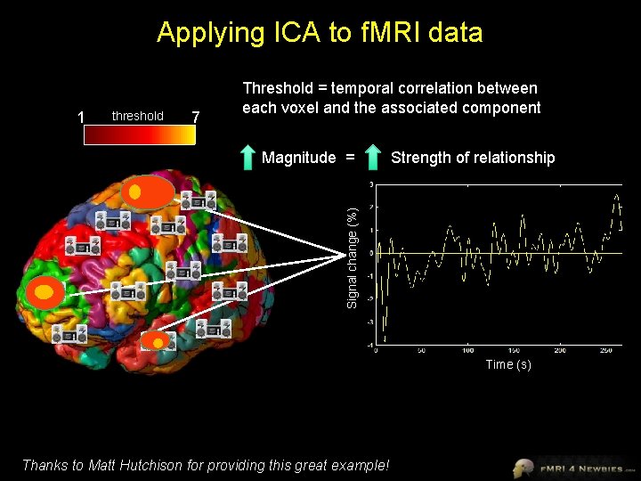
Applying ICA to f. MRI data 1 threshold 7 Threshold = temporal correlation between each voxel and the associated component Strength of relationship Signal change (%) Magnitude = Time (s) Thanks to Matt Hutchison for providing this great example!

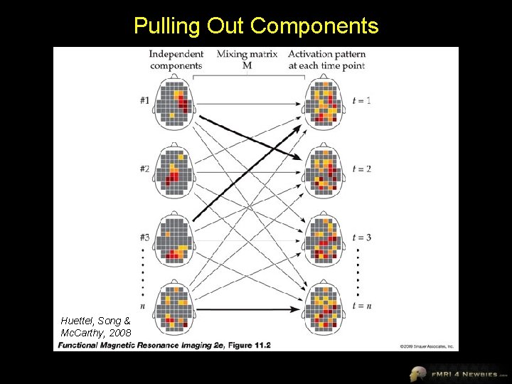
Pulling Out Components Huettel, Song & Mc. Carthy, 2008

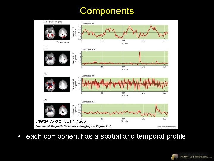
Components Huettel, Song & Mc. Carthy, 2008 • each component has a spatial and temporal profile

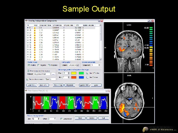
Sample Output

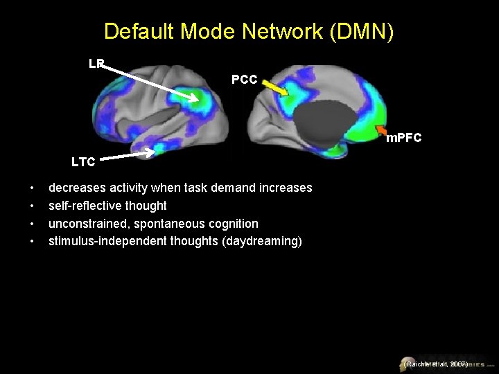
Default Mode Network (DMN) LP PCC m. PFC LTC • • decreases activity when task demand increases self-reflective thought unconstrained, spontaneous cognition stimulus-independent thoughts (daydreaming) (Raichle et al. , 2007)

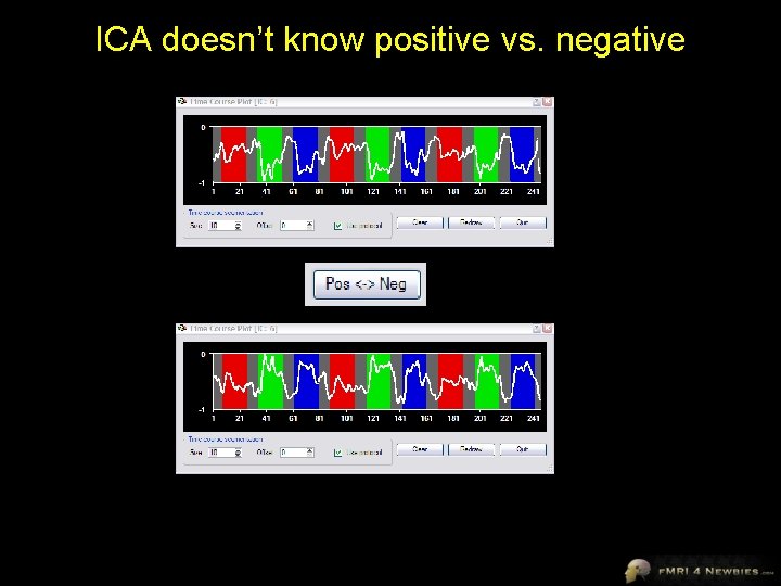
ICA doesn’t know positive vs. negative

Uses of ICA • see if ICA finds components that match your hypotheses – but then why not just use hypothesis-driven approach? • use ICA to remove noise components • use ICA for exploratory analyses – may be especially useful for situations where pattern is uncertain • hallucinations, seizures • use ICA to analyze resting state data – stay tuned till connectivity lecture for more info

Making Sense of Components • how many components? – too many • splitting of components • hard to dig through – too few • clumping of components – 20 -40 recommended – some algorithms can estimate # components • how do you make sense of them? – visual inspection – sorting – fingerprints

Sorting Components • variance accounted for by component • spatial correlation with known areas – regions of interest (e. g. , fusiform face area) – networks of interest (e. g. , default mode network) • temporal correlation with known events – task predictors

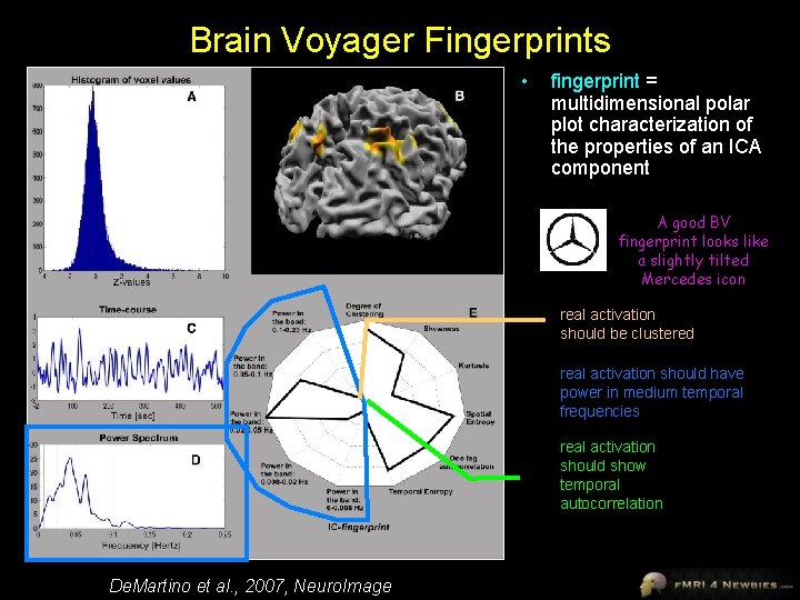
Brain Voyager Fingerprints • fingerprint = multidimensional polar plot characterization of the properties of an ICA component A good BV fingerprint looks like a slightly tilted Mercedes icon real activation should be clustered real activation should have power in medium temporal frequencies real activation should show temporal autocorrelation De. Martino et al. , 2007, Neuro. Image

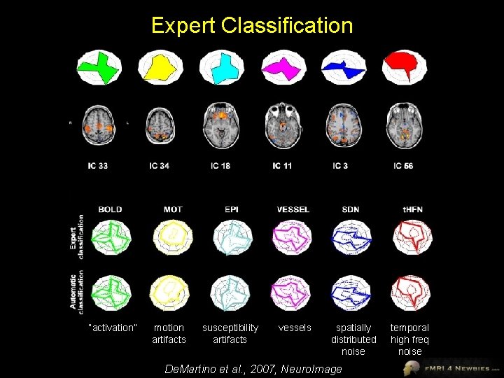
Expert Classification “activation” motion artifacts susceptibility artifacts vessels spatially distributed noise De. Martino et al. , 2007, Neuro. Image temporal high freq noise

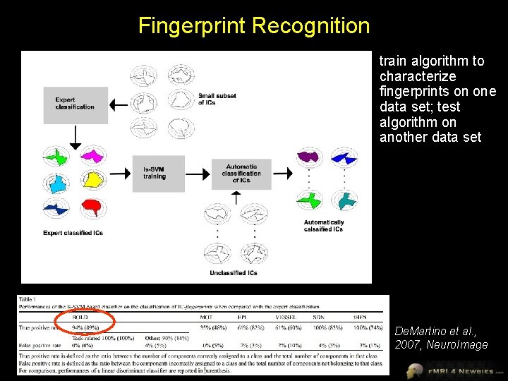
Fingerprint Recognition • train algorithm to characterize fingerprints on one data set; test algorithm on another data set De. Martino et al. , 2007, Neuro. Image

Miscellaneous

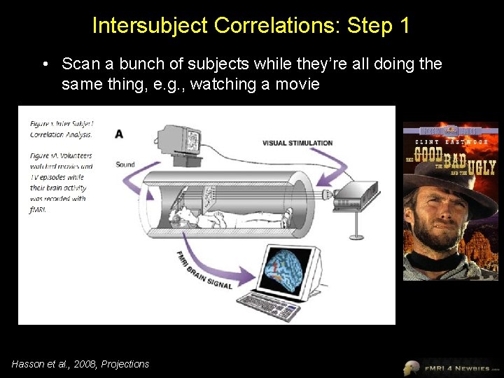
Intersubject Correlations: Step 1 • Scan a bunch of subjects while they’re all doing the same thing, e. g. , watching a movie Hasson et al. , 2008, Projections

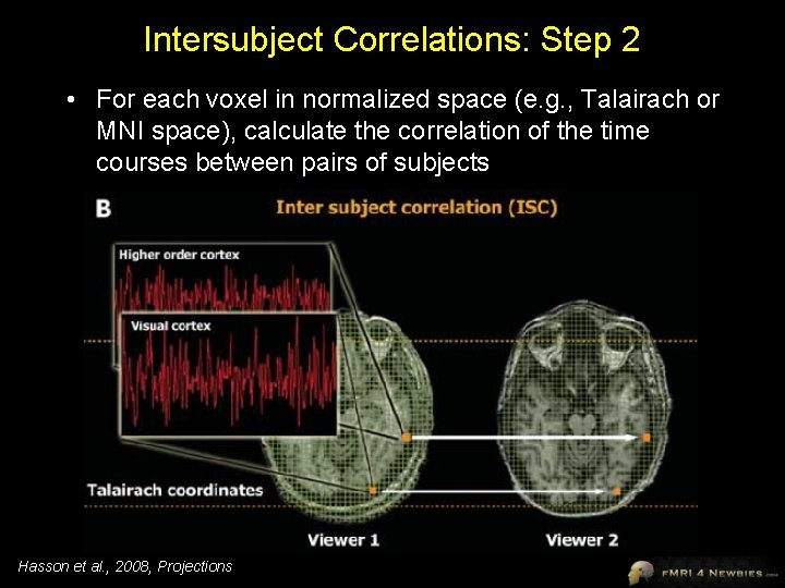
Intersubject Correlations: Step 2 • For each voxel in normalized space (e. g. , Talairach or MNI space), calculate the correlation of the time courses between pairs of subjects Hasson et al. , 2008, Projections

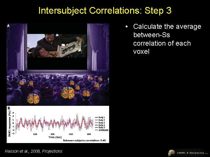
Intersubject Correlations: Step 3 • Calculate the average between-Ss correlation of each voxel Hasson et al. , 2008, Projections

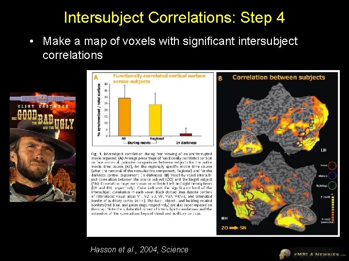
Intersubject Correlations: Step 4 • Make a map of voxels with significant intersubject correlations Hasson et al. , 2004, Science

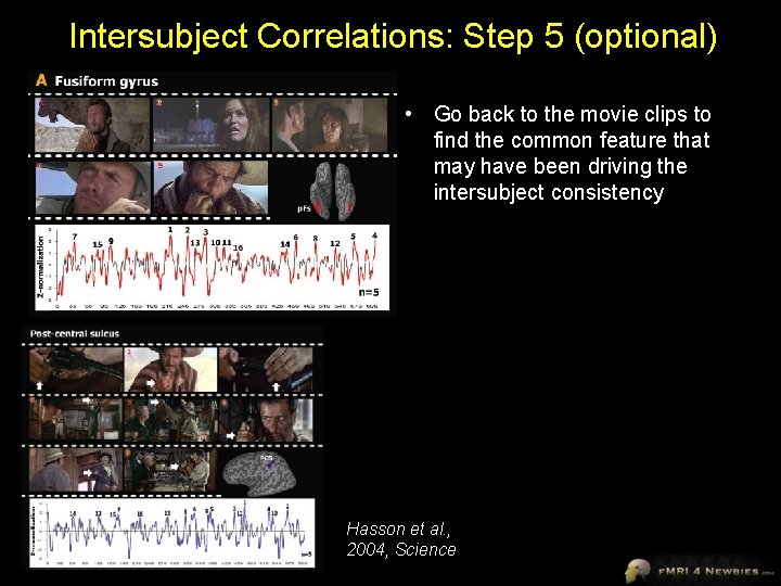
Intersubject Correlations: Step 5 (optional) • Go back to the movie clips to find the common feature that may have been driving the intersubject consistency Hasson et al. , 2004, Science

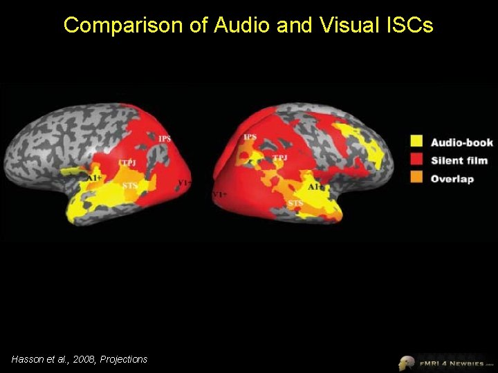
Comparison of Audio and Visual ISCs Hasson et al. , 2008, Projections

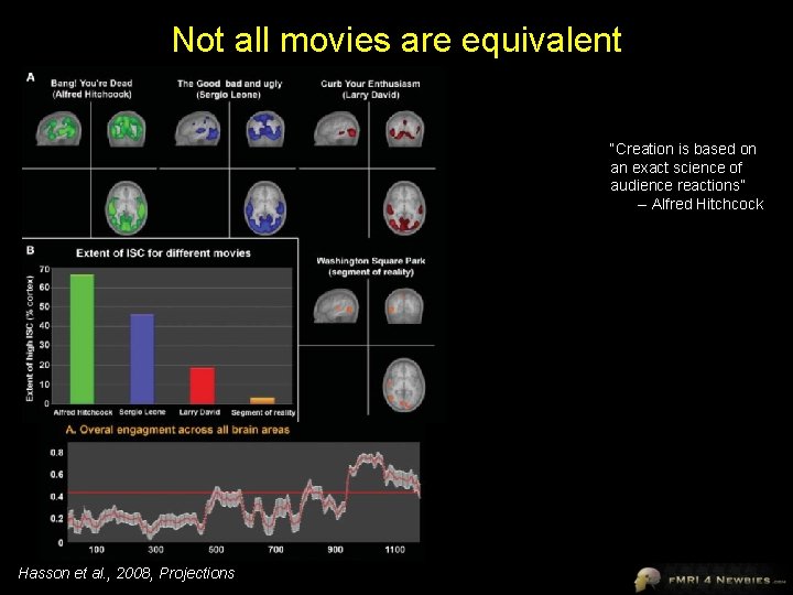
Not all movies are equivalent “Creation is based on an exact science of audience reactions” -- Alfred Hitchcock Hasson et al. , 2008, Projections

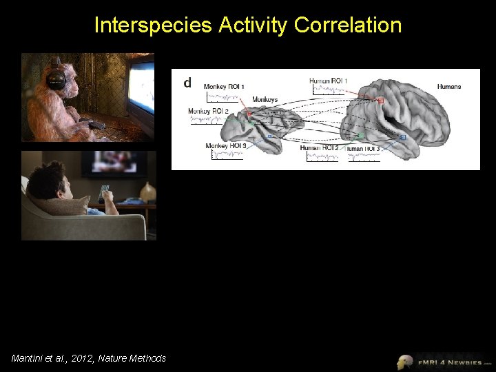
Interspecies Activity Correlation Mantini et al. , 2012, Nature Methods

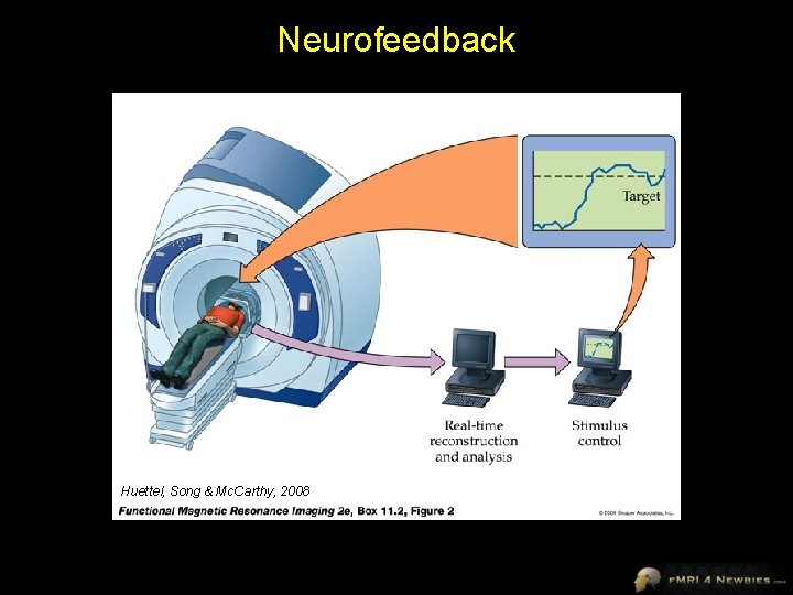
Neurofeedback Huettel, Song & Mc. Carthy, 2008

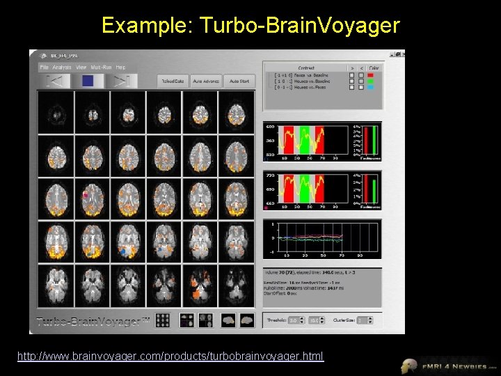
Example: Turbo-Brain. Voyager http: //www. brainvoyager. com/products/turbobrainvoyager. html

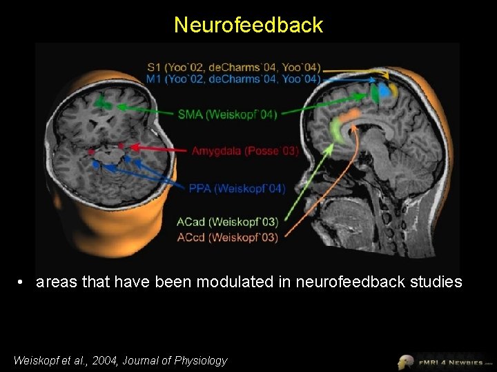
Neurofeedback • areas that have been modulated in neurofeedback studies Weiskopf et al. , 2004, Journal of Physiology

Uses of Real-Time f. MRI • detect artifacts immediately and give subjects feedback • training for brain-computer interfaces • reduce symptoms – e. g. , pain perception • neurocognitive training • ensuring functional localizers worked • studying social interactions

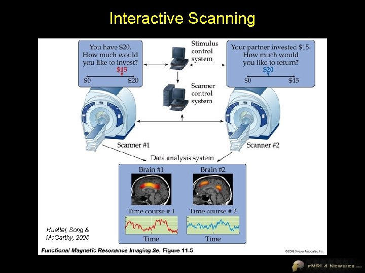
Interactive Scanning Huettel, Song & Mc. Carthy, 2008

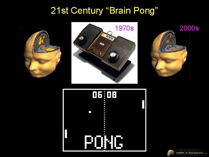
21 st Century “Brain Pong” 1970 s 2000 s