January 2014 IEEE 802 15 14 0052 00

January 2014 IEEE 802. 15 -14 -0052 -00 -004 q Project: IEEE P 802. 15 Working Group for Wireless Personal Area Networks (WPANs) Submission Title: Simulation of flat Ricean fading channel Date Submitted: January 21, 2014 Source: Jinesh P Nair 1, Kiran Bynam 1, Youngsoo Kim 1, , Chandrashekhar Thejaswi PS 1, Frederik Beer 2. 1 Samsung Electronics, 2 FAU/IIS Phone: +918041819999 -464, Fax: +918041819999 E-Mail: jinesh. p@samsung. com Abstract: Description of simulation of flat Ricean fading channel Purpose: Reference on channel models for fair comparison of proposals and system evaluation Notice: This document has been prepared to assist the IEEE P 802. 15. It is offered as a basis for discussion and is not binding on the contributing individual(s) or organization(s). The material in this document is subject to change in form and content after further study. The contributor(s) reserve(s) the right to add, amend or withdraw material contained herein. Release: The contributor acknowledges and accepts that this contribution becomes the property of IEEE and may be made publicly available by P 802. 15. Submission Slide 1 Jinesh P Nair, Kiran Bynam and Youngsoo Kim

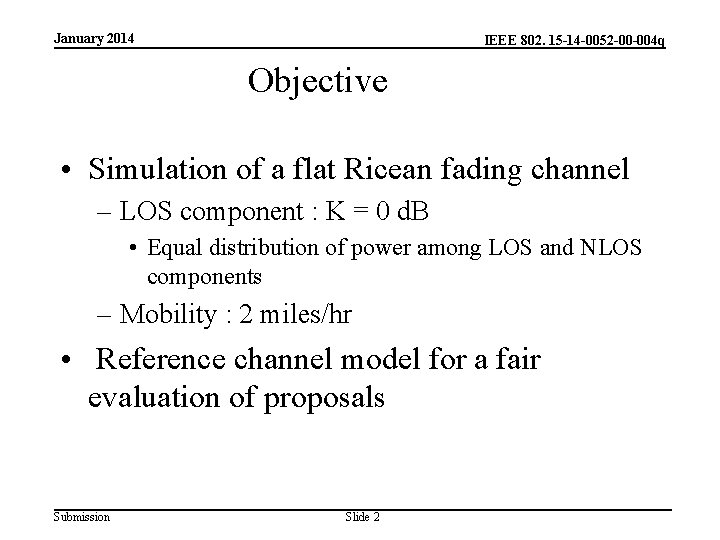
January 2014 IEEE 802. 15 -14 -0052 -00 -004 q Objective • Simulation of a flat Ricean fading channel – LOS component : K = 0 d. B • Equal distribution of power among LOS and NLOS components – Mobility : 2 miles/hr • Reference channel model for a fair evaluation of proposals Submission Slide 2

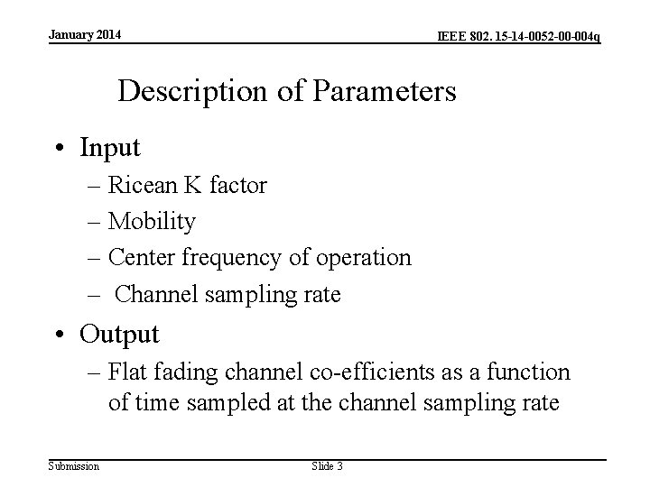
January 2014 IEEE 802. 15 -14 -0052 -00 -004 q Description of Parameters • Input – Ricean K factor – Mobility – Center frequency of operation – Channel sampling rate • Output – Flat fading channel co-efficients as a function of time sampled at the channel sampling rate Submission Slide 3

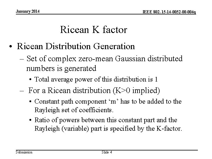
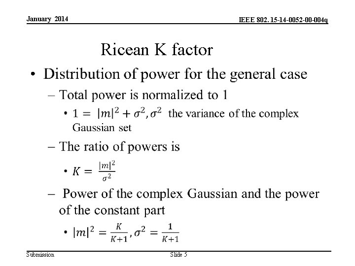
January 2014 IEEE 802. 15 -14 -0052 -00 -004 q Ricean K factor • Ricean Distribution Generation – Set of complex zero-mean Gaussian distributed numbers is generated • Total average power of this distribution is 1 – For a Ricean distribution (K>0 implied) • Constant path component ‘m’ has to be added to the Rayleigh set of coefficients. • Ratio of powers between this constant part and the Rayleigh (variable) part is specified by the K-factor. Submission Slide 4

January 2014 IEEE 802. 15 -14 -0052 -00 -004 q Ricean K factor • Submission Slide 5

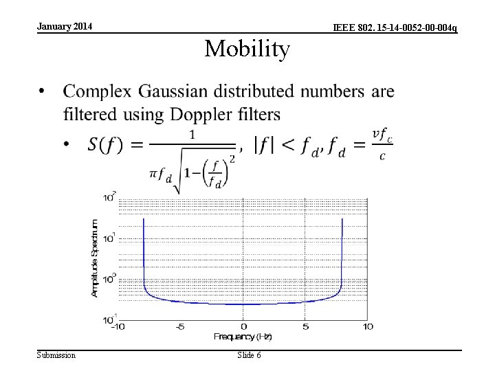
January 2014 IEEE 802. 15 -14 -0052 -00 -004 q Mobility Submission Slide 6

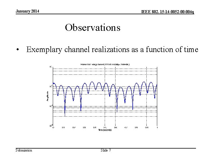
January 2014 IEEE 802. 15 -14 -0052 -00 -004 q Observations • Exemplary channel realizations as a function of time Submission Slide 7

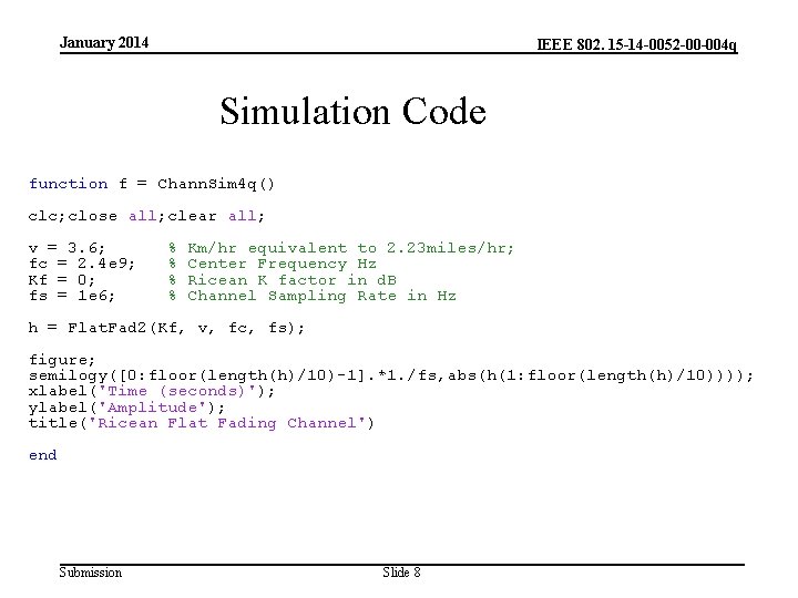
January 2014 IEEE 802. 15 -14 -0052 -00 -004 q Simulation Code function f = Chann. Sim 4 q() clc; close all; clear all; v = 3. 6; fc = 2. 4 e 9; Kf = 0; fs = 1 e 6; % % Km/hr equivalent to 2. 23 miles/hr; Center Frequency Hz Ricean K factor in d. B Channel Sampling Rate in Hz h = Flat. Fad 2(Kf, v, fc, fs); figure; semilogy([0: floor(length(h)/10)-1]. *1. /fs, abs(h(1: floor(length(h)/10)))); xlabel('Time (seconds)'); ylabel('Amplitude'); title('Ricean Flat Fading Channel') end Submission Slide 8

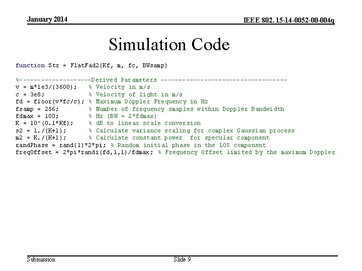
January 2014 IEEE 802. 15 -14 -0052 -00 -004 q Simulation Code function Str = Flat. Fad 2(Kf, m, fc, BWsamp) %----------Derived Parameters -----------------v = m*1 e 3/(3600); % Velocity in m/s c = 3 e 8; % Velocity of light in m/s fd = floor(v*fc/c); % Maximum Doppler Frequency in Hz fsamp = 256; % Number of frequency smaples within Doppler Bandwidth fdmax = 100; % Hz (BW = 2*fdmax) K = 10^(0. 1*Kf); % d. B to linear scale conversion s 2 = 1. /(K+1); % Calculate variance scaling for complex Gaussian process m 2 = K. /(K+1); % Calculate constant power for specular component rand. Phase = rand(1)*2*pi; % Random initial phase in the LOS component freq. Offset = 2*pi*randi(fd, 1, 1)/fdmax; % Frequency Offset limited by the maximum Doppler Submission Slide 9

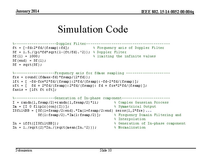
January 2014 IEEE 802. 15 -14 -0052 -00 -004 q Simulation Code %----------Doppler Filter--------------------ft = [-fd: 2*fd/(fsamp): fd]; % Frequency axis of Doppler Filter Sf = 1. 5. /(pi*fd*sqrt(1 -(ft/fd). ^2)); % Doppler Filter Sf(1) = 1000; % limiting the infinite values Sf(end) = Sf(1); Sf = sqrt(Sf); %----------Frequency axis for fdmax sampling ----------fre = round((fdmax-fd)*fsamp/(2*fd)); lft = [ -fd-fre*2*fd/(fsamp): -fd-2*fd/(fsamp)]; rft = [ fd + 2*fd/(fsamp): fd + fre*2*fd/(fsamp)]; faxis = [lft ft rft]; %----------Generation of In-phase component-----------I = randn(1, fsamp/2)+randn(1, fsamp/2)*1 i; % Complex Gaussian Process Im = [I 0 fliplr(conj(I))]; % Symmetrical Output ISfilt. BB = [Sf(1+fsamp/2: end). *Im(1+fsamp/2: end) zeros(1, 2*fre). . . Sf(1: fsamp/2). *Im(1: fsamp/2)]; % Frequency Domain Filtering and % Interpolation In = ifft([ISfilt. BB]); % Generation of In-phase component In = 1. /sqrt(2)*In. /(sqrt(mean(In. ^2))); % Normalization Submission Slide 10

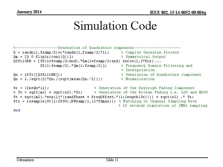
January 2014 IEEE 802. 15 -14 -0052 -00 -004 q Simulation Code %----------Generation of Quadrature component----------Q = randn(1, fsamp/2)+i*randn(1, fsamp/2)*1 i; % Complex Gaussian Process Qm = [Q 0 fliplr(conj(Q))]; % Symmetrical Output QSfilt. BB = [Sf(1+fsamp/2: end). *Qm(1+fsamp/2: end) zeros(1, 2*fre). . . Sf(1: fsamp/2). *Qm(1: fsamp/2)]; % Frequency Domain Filtering and % Interpolation Qn = ifft([QSfilt. BB]); % Generation of Quadrature component Qn = 1. /sqrt(2)*Qn. /(sqrt(mean(Qn. ^2))); % Normalization Sr = (In+Qn*1 i); % Generation of the Rayleigh Fading Component % St = sqrt(m 2) + sqrt(s 2). *Sr; % Generation of the Ricean Fading i. e. LOS and NLOS St = sqrt(m 2). *exp(1 j*(rand. Phase + freq. Offset. *(1: length(Sr)))) + sqrt(s 2). * Sr; Str = resample(St(1: 2000), BWsamp/1, (2*fdmax)); % Matching to Channel Sampling Rate % 10 seconds simulation at 1 MHz sampling end Submission Slide 11

January 2014 IEEE 802. 15 -14 -0052 -00 -004 q References 1. Marco Hernandez et al, “Channel models for TG 8” IEEE P 802. 15 Working Group for Wireless Personal Area Networks (WPANs), Sept 2012 2. Jinesh Nair, Kiran Bynam and Youngsoo Kim, “Channel Models for IEEE 802. 15. 4 q” IEEE P 802. 15 Working Group for Wireless Personal Area Networks (WPANs), DCN: 15 -12 -0329 -00, May. 2013 3. T. Rappaport, “Wireless Communications” Pearson Education, 2 nd Edition, 2002. Submission Slide 12