Jacek Wallusch Statistics for International Business Lecture 3

Jacek Wallusch _________________ Statistics for International Business Lecture 3: Skewness and Kurtosis

graphical presentation Shape of distribution ______________________________________________ Skewness: measures the skewness of a distribution; positive or negative skewness Kurtosis: measures the peackedness of a distribution; leptokurtic (positive excess kurtosis, i. e. fatter tails), tails mesokurtic, platykurtic (negative excess kurtosis, i. e. thinner tails), tails Statistics: 3 fat tails – to be found in e. g. recent financial econometrics and chaotic dynamics

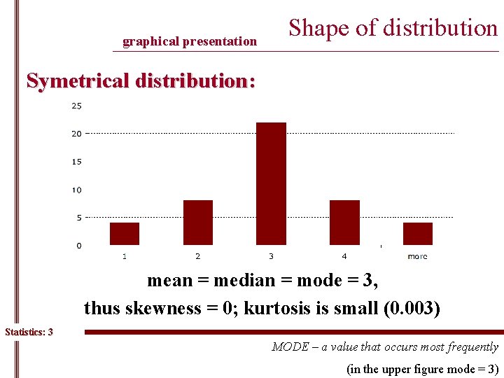
graphical presentation Shape of distribution ______________________________________________ Symetrical distribution: mean = median = mode = 3, thus skewness = 0; kurtosis is small (0. 003) Statistics: 3 MODE – a value that occurs most frequently (in the upper figure mode = 3)

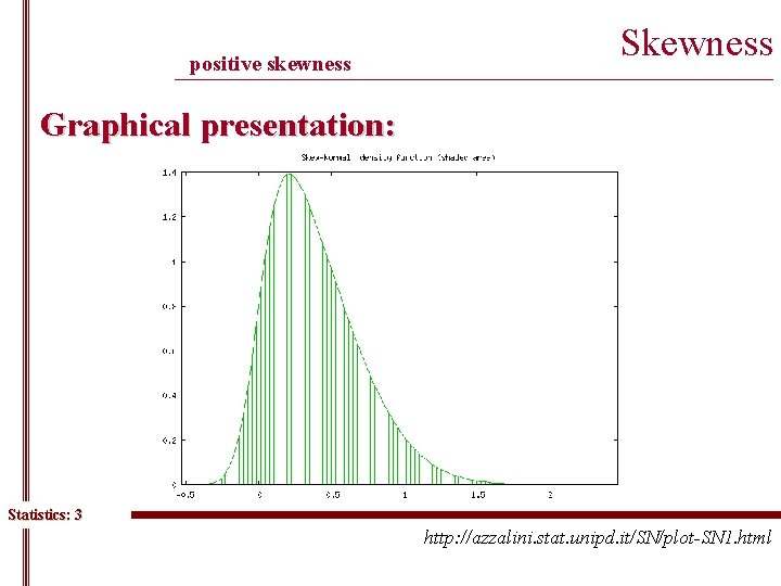
positive skewness Skewness ______________________________________________ Graphical presentation: Statistics: 3 http: //azzalini. stat. unipd. it/SN/plot-SN 1. html

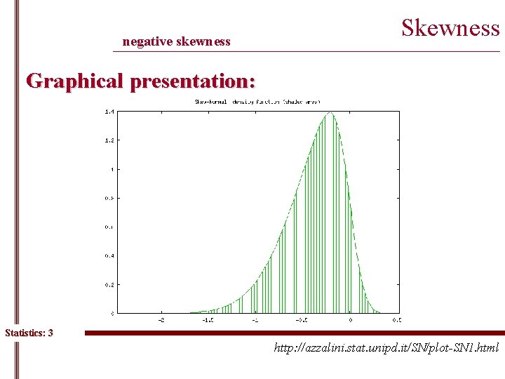
negative skewness Skewness ______________________________________________ Graphical presentation: Statistics: 3 http: //azzalini. stat. unipd. it/SN/plot-SN 1. html

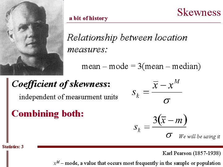
a bit of history Skewness __________________________________________ Relationship between location measures: mean – mode = 3(mean – median) Coefficient of skewness: independent of measurment units Combining both: We will be using it Statistics: 3 Karl Pearson (1857 -1938) x. M – mode, a value that occurs most frequently in the sample or population

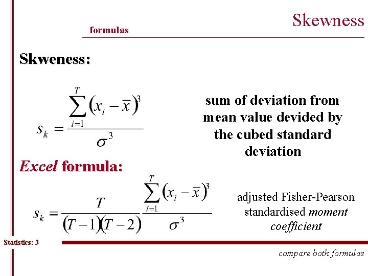
formulas Skewness ______________________________________________ Skweness: Excel formula: sum of deviation from mean value devided by the cubed standard deviation adjusted Fisher-Pearson standardised moment coefficient Statistics: 3 compare both formulas

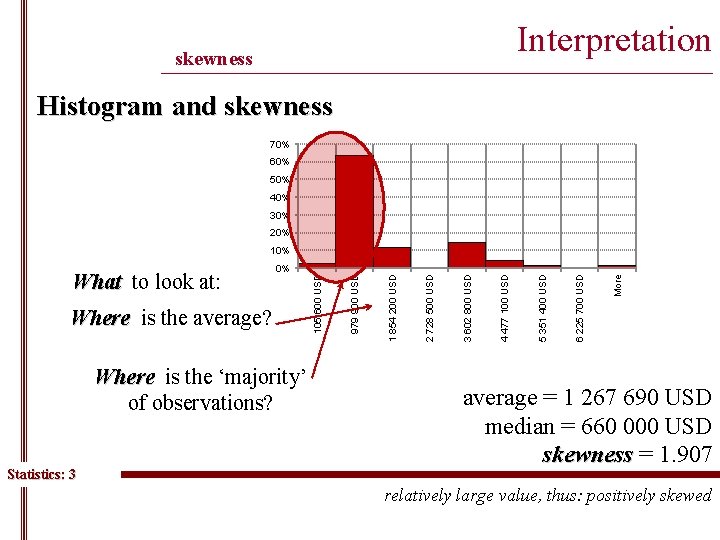
Interpretation skewness ______________________________________________ Histogram and skewness 70% 60% 50% 40% 30% 20% Where is the ‘majority’ of observations? Statistics: 3 More 6 225 700 USD 5 351 400 USD 4 477 100 USD 3 602 800 USD 2 728 500 USD 1 854 200 USD Where is the average? 979 900 USD What to look at: 0% 105 600 USD 10% average = 1 267 690 USD median = 660 000 USD skewness = 1. 907 relatively large value, thus: positively skewed

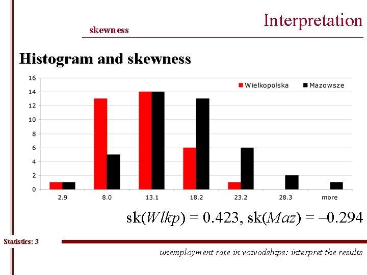
Interpretation skewness ______________________________________________ Histogram and skewness sk(Wlkp) = 0. 423, sk(Maz) = – 0. 294 Statistics: 3 unemployment rate in voivodships: interpret the results

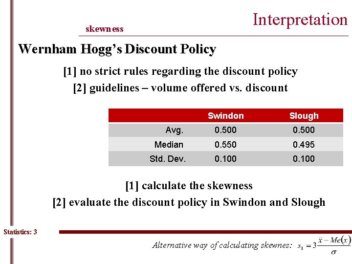
Interpretation skewness ______________________________________________ Wernham Hogg’s Discount Policy [1] no strict rules regarding the discount policy [2] guidelines – volume offered vs. discount Swindon Slough Avg. 0. 500 Median 0. 550 0. 495 Std. Dev. 0. 100 [1] calculate the skewness [2] evaluate the discount policy in Swindon and Slough Statistics: 3 Alternative way of calculating skewnes:

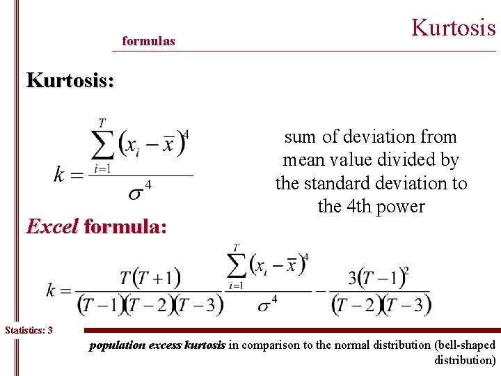
formulas Kurtosis ______________________________________________ Kurtosis: Excel formula: sum of deviation from mean value divided by the standard deviation to the 4 th power Statistics: 3 population excess kurtosis in comparison to the normal distribution (bell-shaped distribution)

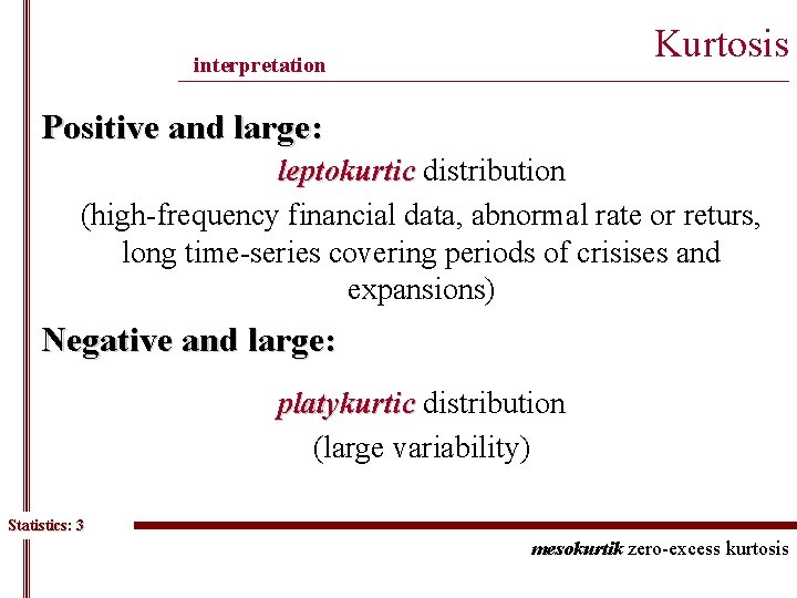
Kurtosis interpretation ______________________________________________ Positive and large: leptokurtic distribution (high-frequency financial data, abnormal rate or returs, long time-series covering periods of crisises and expansions) Negative and large: platykurtic distribution (large variability) Statistics: 3 mesokurtik zero-excess kurtosis

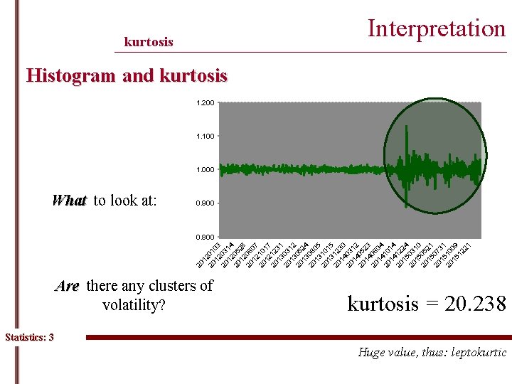
Interpretation kurtosis ______________________________________________ Histogram and kurtosis 1. 200 1. 100 1. 000 What to look at: 0. 900 20 12 20 01 12 03 20 03 12 14 20 05 12 28 20 08 12 07 20 10 12 17 20 12 13 31 20 03 13 12 20 05 13 24 20 08 13 05 20 10 13 15 20 12 14 30 20 03 14 12 20 05 14 23 20 08 14 04 20 10 14 14 20 12 15 24 20 03 15 10 20 05 15 21 20 07 15 31 20 10 15 09 12 21 0. 800 Are there any clusters of volatility? kurtosis = 20. 238 Statistics: 3 Huge value, thus: leptokurtic

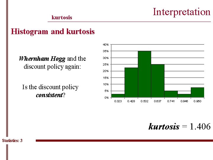
Interpretation kurtosis ______________________________________________ Histogram and kurtosis 40% 35% Whernham Hogg and the discount policy again: 30% 25% 20% 15% Is the discount policy consistent? consistent 10% 5% 0% 0. 323 0. 428 0. 532 0. 637 0. 741 0. 846 0. 950 kurtosis = 1. 406 Statistics: 3

one week to 1 st. mid-term Repetition ______________________________________________ Arithmetic mean; Geometric mean; Weighted average; Variance; Standard deviation; Statistics: 3 when to use them? how to interpret them? how to calculate the weights? how to interpret? how to detect outliers?

one week to 1 st. mid-term Repetition ______________________________________________ Skewness; Kurtosis; how to interpret? Histogram; Ogive; Statistics: 3 relation to measures of location, dispersion, skewness and kurtosis