IV MULTIPLE LOGISTIC REGRESSION v Extend simple logistic

IV. MULTIPLE LOGISTIC REGRESSION v Extend simple logistic regression to models with multiple covariates v Similarity between multiple linear and multiple logistic regression v Multiple 2 x 2 tables and the Mantel-Haenszel test Ø Estimating an odds ratio that is adjusted for a confounding variable v Using logistic regression as an alternative to the Mantel-Haenszel test v Using indicator covariates to model categorical variables v Making inferences about odds ratios derived from multiple parameters v Analyzing complex data with logistic regression Ø Multiplicative models Ø Models with interaction v Assessing model fit Ø Testing the change in model deviance in nested models Ø Evaluating residuals and influence v Using restricted cubic splines in logistic regression models Ø Plotting the probability of an outcome with confidence bands Ø Plotting odds ratios and confidence bands © William D. Dupont, 2010, 2011 Use of this file is restricted by a Creative Commons Attribution Non-Commercial Share Alike license. See http: //creativecommons. org/about/licenses for details.

1. The Model If the data is organized as one record per patient then the model is {4. 1} logit where xi 1, x 12, …, xik are covariates from the ith patient , 1, . . . k, are unknown parameters di = 1: 0: ith patient suffers event of interest otherwise

If the data is organized as one record per unique combination of covariate values then the model is logit {4. 2} where mi is the number of patients with covariate values xi 1, xi 2, …, xik and di is the number of events among these mi subjects. di is assumed to have a binomial distribution obtained from mi dichotomous trials with probability of success on each trial. Thus, the only difference between simple and multiple logistic regression is that the linear predictor is now . As in simple logistic regression, the model has a logit link function; the random component, di/mi has a binomial distribution.

2. Mantel-Haenszel Test of a Common Odds Ratio The following data is from the Ille-et-Vilaine study of esophageal cancer and alcohol by Tuyns et al. (1977). This data is published in Appendix I of Breslow and Day Vol. I, who also provide an excellent and extensive discussion of this data set.

Cancer Age 25 -34 35 -44 45 -54 55 -64 65 -74 Yes No Yes No Daily Alcohol Consumption > 80 g <80 g % > 80 g 1 9 0 106 1 100. 00% 115 7. 83% 10 106 116 8. 62% 4 26 5 164 9 190 44. 44% 13. 68% 30 169 199 15. 08% 25 29 21 138 46 167 54. 35% 17. 37% 54 159 213 25. 35% 42 27 34 139 76 166 55. 26% 16. 27% 69 173 242 28. 51% 19 18 36 88 55 106 34. 55% 16. 98% 37 124 161 22. 98%

a) Confounding Variables A confounding variable is one that is associated with both the disease and exposure of interest but which is not, in itself, a focus of our investigation. Note mild evidence that age confounds the effect of alcohol on cancer risk. b) Age-adjusted odds ratios The following log file show to calculate the common odds ratio for esophageal cancer associated with heavy alcohol use in five age strata. It thus calculates an age-adjusted odds ratio for esophageal cancer among heavy and light drinkers of similar age.

3. Deriving the Mantel-Haenszel test with Stata * 5. 5. Esophageal. Ca. log. *. * Calculate the Mantel-Haenszel age-adjusted odds ratio from. * the Ille-et-Vilaine study of esophageal cancer and alcohol. * (Breslow & Day 1980, Tuyns 1977). . *. use C: WDDtext5. 5. Esophageal. Ca. dta, clear . codebook age cancer heavy age --------------------- Age (years) type: numeric (float) label: age range: [1, 6] units: 1 unique values: 6 coded missing: 0 / 192 tabulation: Freq. Numeric Label 32 1 25 -34 32 2 35 -44 32 3 45 -54 32 4 55 -64 32 5 65 -74 32 6 >= 75

cancer ---------------- Esophageal Cancer type: numeric (float) label: yesno range: [0, 1] units: 1 unique values: 2 coded missing: 0 / 192 tabulation: Freq. Numeric Label 96 0 No 96 1 Yes heavy ------------- Heavy Alcohol Consumption type: numeric (float) label: heavy range: [0, 1] units: 1 unique values: coded missing: 0 / 192 tabulation: Freq. Numeric Label 96 0 < 80 gm 96 1 >= 80 gm

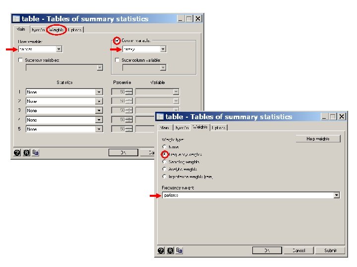
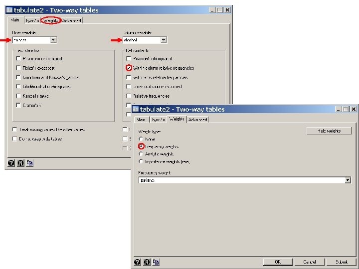
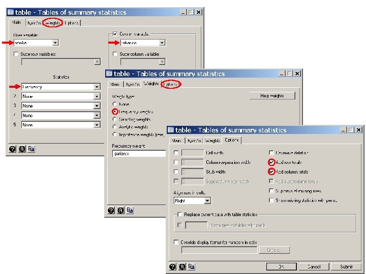
. * Statistics > Summaries. . . > Tables > Table of summary statistics (table). table heavy cancer [freq=patients] {1} -----+--------- | Heavy Alcohol Esophagea | Consumption l Cancer | < 80 gm >= 80 gm -----+--------- No | 666 104 Yes | 109 96 -----+--------- {1} This table command gives 2 2 cross-tables of heavy by cancer, and confirms that Esophageal. Cancer. dta is the correct data set.

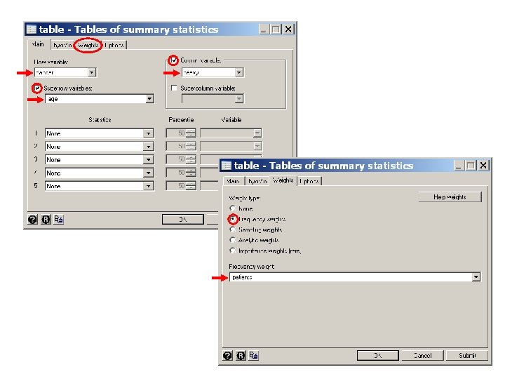
. table cancer heavy [freq=patients], by(age) -----+---------Age | (years) | and | Heavy Alcohol Esophagea | Consumption l Cancer | < 80 gm >= 80 gm -----+---------25 -34 | No | 106 9 Yes | 1 -----+---------35 -44 | No | 164 26 Yes | 5 4 -----+---------45 -54 | No | 138 29 Yes | 21 25 -----+---------55 -64 | No | 139 27 Yes | 34 42 -----+---------65 -74 | No | 88 18 Yes | 36 19 -----+--------->= 75 | No | 31 Yes | 8 5 -----+----------

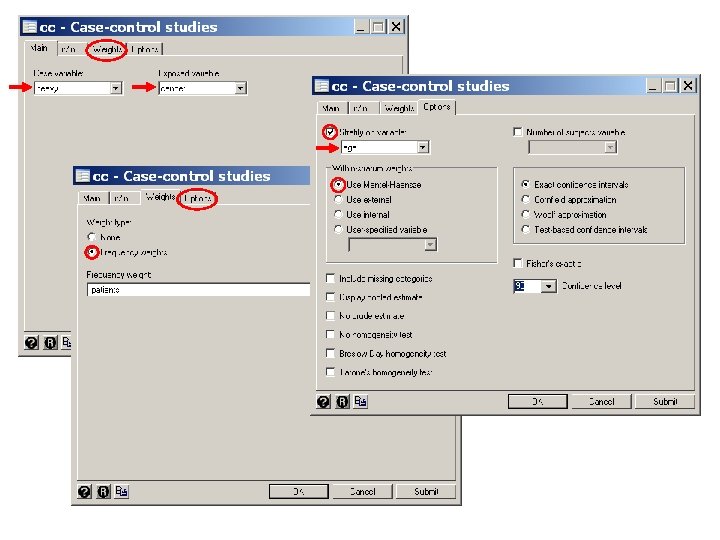
. * Statistics > Epidemiology. . . > Tables. . . > Case-control odds ratio. cc heavy cancer [freq=patients], by(age) Age (years) | OR [95% Conf. Interval] M-H Weight -------+------------------------ 25 -34 | . 0 (exact) 35 -44 | 5. 046154 . 9268664 24. 86538 . 6532663 (exact) 45 -54 | 5. 665025 2. 632894 12. 16536 2. 859155 (exact) 55 -64 | 6. 359477 3. 299319 12. 28473 3. 793388 (exact) 65 -74 | 2. 580247 1. 131489 5. 857261 4. 024845 (exact) >= 75 | . 4. 388738 . 0 (exact) -------+------------------------ Crude | 5. 640085 3. 937435 8. 061794 (exact) M-H combined | 5. 157623 3. 562131 7. 467743 -------+------------------------Test of homogeneity (Tarone) chi 2(5) = 9. 30 Pr>chi 2 = 0. 0977 Test that combined OR = 1: Mantel-Haenszel chi 2(1) = 85. 01 Pr>chi 2 = 0. 0000 {2} {3} {4} {5} {6}

{2} The by(age) option causes odds ratios to be calculated for each age strata. No estimate is given for the youngest strata because there were no moderate drinking cases. No estimate is given for the oldest strata because there were no heavy drinking controls.

The M-H estimate is only reasonable if the data is consistent with the hypothesis that the alcohol-cancer odds ratio does not vary with age. The test for homogeneity tests the null hypothesis that all age strata share a common odds ratio. This test is not significant, which suggests that the M-H estimate may be reasonable. {5} {6} The test of the null hypotheses that the odds ratio equals 1 is highly significant. Hence the association between heavy alcohol consumption and esophageal cancer can not be explained by chance. The argument for a causal relationship is strengthened by the magnitude of the odds ratio.

4. Effect Modifiers and Confounding Variables a) Test of homogeneity of odds ratios In the previous example the test for homogeneity of the odds ratio was not significant (see comment 5). Of course, lack of significance does not prove the null hypotheses, and it is prudent to look at the odds ratios from the individual age strata. In the preceding Stata output these values are fairly similar for all strata except ages 65 -74, where the odds ratio drops to 2. 6. This may be due to chance, or perhaps, to a hardy survivor effect. You must use your clinical judgment in deciding what to report. Effect Modifier: A variable that influences the effect of a risk factor on the outcome variable. The key differences between confounding variables and effect modifiers are: i) Confounding variables are not of primary interest in our study while effect modifiers are. ii) A variable is an important effect modifier if there is a meaningful interaction between it and the exposure of interest on the risk of the event under study.

5. Logistic Regression For Multiple 2× 2 Contingency Tables a) Estimating the common relative risk from the parameter estimates Let mjk be the number of subjects in the jth age strata who are (k = 1) or not (k = 0) heavy drinkers. djk be the number of cancers among these mjk subjects. xk = k = 1 or 0 depending on their drinking status. jk be the probability that someone in the jth age strata who 1) or doesn’t (k = 0) drink heavily develops cancer. does (k = are

Consider the logistic regression model {4. 3} logit where djk has a binomial distribution obtained from mjk independent trials with probability of success with jk on each trial. Then for any age strata j, and logit {4. 4} Similarly logit {4. 5} Subtracting equation {4. 4} from equation {4. 5} gives that log or

Hence, this model implies that the odds ratio for cancer is the same in all strata and equals exp( ). This is an age-adjusted estimate of the cancer odds ratio In practice we fit model {4. 1} by defining indicator covariates zj = 1: if subjects are from the jth age strata 0: otherwise Then {4. 3} becomes

Note that this model places no restraints of the effect of age on the odds of cancer and only requires that the within strata odds ratio be constant. For example, a moderate drinker from the 3 rd age stratum has log odds While a moderate drinker from the first age stratum has Hence the log odds ratio for stratum 3 versus stratum 1 is 3 - 1, which can be estimated independently of the cancer risk associated with age strata 2, 4, 5 and 6.

An equivalent model is dc logit E d jk / m jk hi = a +z 2 a 2 +z 3 a 3 +z 4 a 4 +z 5 a 5 +z 6 a 6 +x k b For this model, a moderate drinker from the 3 rd age stratum has log odds While a moderate drinker from the first age stratum has Hence the log odds ratio for stratum 3 versus stratum 1 is This is slightly preferable to our previous formulation in that it involves one parameter rather than 2. {4. 6}

An alternative model that we could have used is However, this model imposes a linear relationship between age and the log odds for cancer. That is, the log odds ratio for age stratum 2 vs stratum 1 is 2 - = for age stratum 3 vs stratum 1 is 3 - = 2 for age stratum 6 vs stratum 1 is 6 - = 5

6. Analyzing Multiple 2 2 Contingency Tables. * 5. 9. Esophageal. Ca. Class. Version. log. *. * Calculate age-adjusted odds ratio from the Ille-et-Vilaine study. * of esophageal cancer and alcohol using logistic regression. . *. use C: WDDtext5. 5. Esophageal. Ca. dta, clear. *. * First, define indicator variables for the age strata 2 through 6. *

. generate age 2 = 0. replace age 2 = 1 if age == 2 (32 real changes made). generate age 3 = 0. replace age 3 = 1 if age == 3 (32 real changes made). generate age 4 = 0. replace age 4 = 1 if age == 4 (32 real changes made). generate age 5 = 0. replace age 5 = 1 if age == 5 (32 real changes made). generate age 6 = 0. replace age 6 = 1 if age == 6 (32 real changes made)

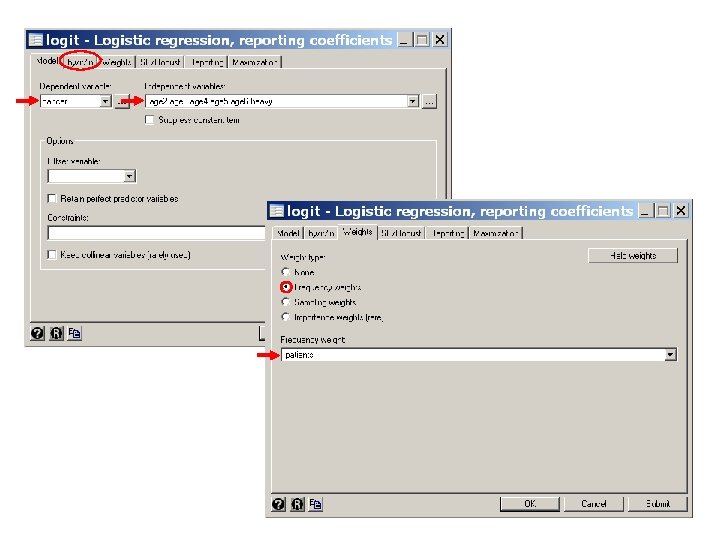
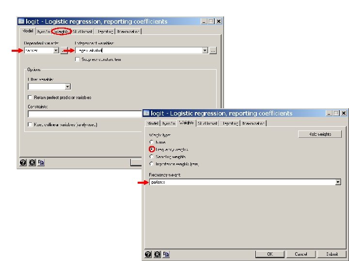
. * Statistics > Binary outcomes > Logistic regression. logit cancer age 2 age 3 age 4 age 5 age 6 heavy [freq=patients] {1} Logistic regression No. of obs = 975 LR chi 2(6) = 200. 57 Prob > chi 2 = 0. 0000 Log likelihood = -394. 46094 Pseudo R 2 = 0. 2027 ------------------------------------cancer | Coef. Std. Err. z P>|z| [95% Conf. Interval] -------+-------------------------------- age 2 | 1. 542294 1. 065895 1. 45 0. 148 -. 546822 3. 63141 age 3 | 3. 198762 1. 02314 3. 13 0. 002 1. 193445 5. 204079 age 4 | 3. 71349 1. 018531 3. 65 0. 000 1. 717207 5. 709774 age 5 | 3. 966882 1. 023072 3. 88 0. 000 1. 961698 5. 972066 age 6 | 3. 96219 1. 065024 3. 72 0. 000 1. 87478 6. 049599 heavy | 1. 66989 . 1896018 8. 81 0. 000 1. 298277 2. 041503 {2} _cons | -5. 054348 1. 009422 -5. 01 0. 000 -7. 032778 -3. 075917 ------------------------------------ The results of this logistic regression are similar to those obtained form the Mantel-Haenszel test. The age-adjusted odds ratio from this latter test was 5. 16 as compared to 5. 31 from logistic regression.

{1} By default, Stata adds a constant term to the model. Hence, this command uses model {4. 6}. The coef option specifies that the model parameter estimates are to be listed as follows. {2} The parameter estimate associated with heavy is 1. 67 with a standard error of 0. 1896. A 95% confidence interval for this interval is 1. 67 + 1. 96 x 0. 1896 = [1. 30, 2. 04]. The age-adjusted estimated odds ratio for cancer in heavy drinkers relative to moderate drinkers is with a 95% confidence interval [exp(1. 30), exp(2. 04)] = [3. 66, 7. 70].

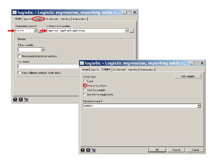
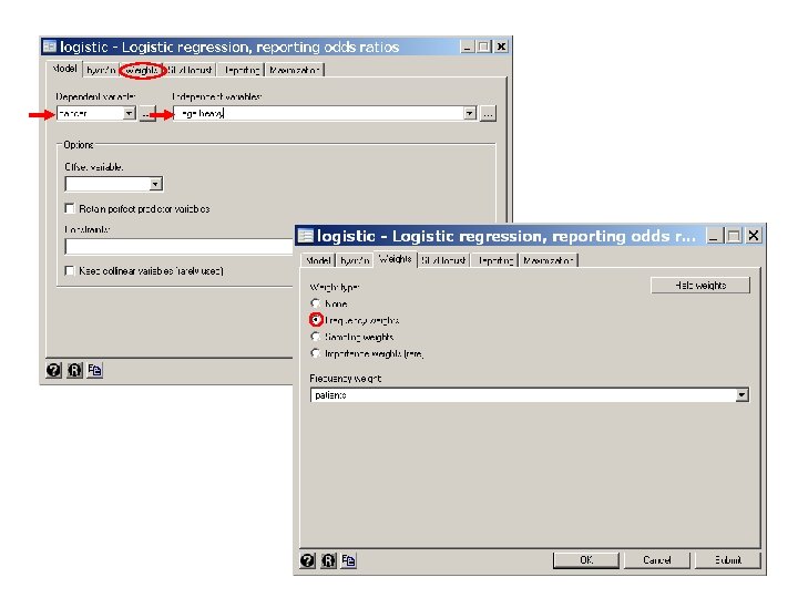
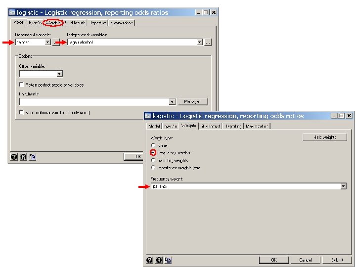
. * Statistics > Binary outcomes > Logistic regression (reporting odds ratios). logistic cancer age 2 age 3 age 4 age 5 age 6 heavy > [freq=patients] {3} Logistic regression No. of obs = 975 LR chi 2(6) = 200. 57 Prob > chi 2 = 0. 0000 Log likelihood = -394. 46094 Pseudo R 2 = 0. 2027 --------------------------------------- cancer | Odds Ratio Std. Err. z P>|z| [95% Conf. Interval] -----+---------------------------------- age 2 | 4. 675303 4. 983382 1. 45 0. 148 . 5787862 37. 76602 age 3 | 24. 50217 25. 06914 3. 13 0. 002 3. 298423 182. 0131 age 4 | 40. 99664 41. 75634 3. 65 0. 000 5. 56895 301. 8028 age 5 | 52. 81958 54. 03823 3. 88 0. 000 7. 777389 392. 3155 age 6 | 52. 57232 55. 99081 3. 72 0. 000 6. 519386 423. 9432 heavy | 5. 311584 1. 007086 8. 81 0. 000 3. 662981 7. 702174 --------------------------------------- {3} Without the coef option logistic does not output the constant parameter and exponentiates the other coefficients. This usually saves hand computation. Note that the age adjusted odds ratio for heavy drinking is 5. 31 with a 95% confidence interval of [3. 7 – 7. 7].

7. Handling Categorical Variables in Stata In the preceding example, age is a categorical variable taking 6 values that is recorded as 5 separate indicator variables. It is very common to recode categorical variables in this way to avoid forcing a linear relationship on the effect of a variable on the response outcome. In the preceding example we did the recording by hand. It can also be done much faster using the i. varname syntax. We illustrate this by repeating the preceding analysis of model {4. 3}. . * Statistics > Binary outcomes > Logistic regression (reporting odds ratios). logistic cancer i. age heavy [freq=patients] {1} Logistic regression No. of obs = 975 LR chi 2(6) = 200. 57 Prob > chi 2 = 0. 0000 Log likelihood = -394. 46094 Pseudo R 2 = 0. 2027 {1} i. age indicates that age is to be recoded as five indicator variables (one for each value of age). These variables are named 2. age, 3. age, 4. age, 5. age, and 6. age. By default the smallest value of age is not assigned a separate indicator variable and a constant term is included in the model giving logit

--------------------------------------- cancer | Odds Ratio. Std. Err. z P>|z| [95% Conf. Interval] -------+-------------------------------- age | 2 | 4. 675303 4. 983382 1. 45 0. 148 . 5787862 37. 76602 3 | 24. 50217 25. 06914 3. 13 0. 002 3. 298423 182. 0131 4 | 40. 99664 41. 75634 3. 65 0. 000 5. 56895 301. 8028 5 | 52. 81958 54. 03823 3. 88 0. 000 7. 111389 392. 3155 6 | 52. 57232 55. 99081 3. 72 0. 000 6. 519386 423. 9432 heavy | 5. 311584 1. 007086 8. 81 0. 000 3. 662981 7. 702174 {2} --------------------------------------- {2} Note that the odds ratio estimate for heavy = 5. 31 is the same as in the earlier analysis where the indicator variables were explicitly defined.

8. Example: Effect of Dose of Alcohol and Tobacco on Esophageal Cancer Risk The Ille-et-Vilaine data set provides four different levels of consumption for both alcohol and tobacco. To investigate the joint effects of dose and alcohol on esophageal cancer risk we first tabulate the raw data. . * 5. 11. 1. Esophageal. Ca. Class. Version. log. *. * Estimate age-adjusted risk of esophageal cancer due to dose of alcohol. . *. use C: WDDtext5. 5. Esophageal. Ca. dta, clear. * Show frequency tables of effect of dose of alcohol on esophageal cancer. . *

. * Statistics > Summaries. . . > Tables > Two-way tables with measures. . tabulate cancer alcohol [freq=patients] , column +----------+ | Key | |----------| | frequency | | column percentage | +----------+ Esophageal | Alcohol (gm/day) Cancer | 0 -39 40 -79 80 -119 >= 120 | Total ------+------------------+------- No | 386 280 87 22 | 775 | 93. 01 78. 87 63. 04 32. 84 | 79. 49 ------+------------------+------- Yes | 29 75 51 45 | 200 | 6. 99 21. 13 36. 96 67. 16 | 20. 51 ------+------------------+------- Total | 415 355 138 67 | 975 | 100. 00 | 100. 00 {1}

. * Statistics > Binary outcomes > Logistic regression. logit cancer i. age i. alcohol [freq=patients] Logit estimates No. of obs = 975 LR chi 2(8) = 274. 07 Prob > chi 2 = 0. 0000 Log likelihood = -363. 7080768 Pseudo R 2 = 0. 2649 --------------------------------------- cancer | Coef. Std. Err. z P>|z| [95% Conf. Interval] -------+-------------------------------- age | 2 | 1. 631112 1. 080013 1. 51 0. 131 -. 4856742 3. 747899 3 | 3. 425834 1. 038937 3. 30 0. 001 1. 389555 5. 462114 4 | 3. 943447 1. 034622 3. 81 0. 000 1. 915624 5. 971269 5 | 4. 356767 1. 041336 4. 18 0. 000 2. 315786 6. 397747 6 | 4. 424219 1. 0914 4. 05 0. 000 2. 285115 6. 563324 | alcohol | 2 | 1. 43431 . 2447858 5. 86 0. 000 . 9545384 1. 914081 {2} 3 | 2. 00711 . 2776153 7. 23 0. 000 1. 462994 2. 551226 4 | 3. 680012 . 3763372 9. 78 0. 000 2. 942405 4. 417619 | _cons | -6. 147181 1. 041877 -5. 90 0. 000 -8. 189223 -4. 10514 ---------------------------------------

{2} The parameter estimates of 2. alcohol, 3. alcohol and 4. alcohol estimate the log-odds ratio for cancer associated with alcohol doses of 40 -79 gm/day, 80 -119 gm/day and 120+ gm/day, respectively. These log-odds ratios are derived with respect to people who drank 0 -39 grams a day. They are all adjusted for age. All of these statistics are significantly different from zero (P<0. 0005).

. * Statistics > Postestimation > Linear combinations of estimates. lincom 3. alcohol - 2. alcohol, or {3} ( 1) - [cancer] 2. alcohol + [cancer]3. alcohol = 0. 0 --------------------------------------- cancer | Odds Ratio Std. Err. z P>|z| [95% Conf. Interval] -------+-------------------------------- (1) | 1. 773226 . 4159625 2. 44 0. 015 1. 119669 2. 808268 --------------------------------------- {3} In general, lincom calculates any linear combination of parameter estimates, tests the null hypothesis that the true value of this combination equals zero, and gives a 95% confidence interval for this estimate. The or option exponentiates the linear combination and calculates the corresponding confidence interval. In this example 3. alcohol – 2. alcohol equals the log-odds ratio for cancer associated with drinking 8 -119 gm/day compared to 40 -79 gm/day. 3. alcohol – 2. alcoh = 2. 001 – 1. 434 = 0. 573, which is significantly different from zero with P = 0. 015. The corresponding odds ratio is exp[0. 573] = 1. 77. The 95% confidence interval for this difference is 2. 8). (1. 1 – Note that the null hypothesis that a log-odds ratio equals zero is equivalent to the null hypothesis that the corresponding odds ratio equals one.

. lincom 4. alcohol - 3. alcohol, or ( 1) [cancer]3. alcohol + [cancer]4. alcohol = 0 --------------------------------------- cancer | Odds Ratio Std. Err. z P>|z| [95% Conf. Interval] -------+-------------------------------- (1) | 5. 327606 1. 95176 4. 57 0. 000 2. 598339 10. 92367 ---------------------------------------

. * Statistics > Binary outcomes > Logistic regression (reporting odds ratios). logisitc cancer i. age i. alcohol [freq=patients] {4} Logit estimates No. of obs = 975 LR chi 2(8) = 274. 07 Prob > chi 2 = 0. 0000 Pseudo R 2 = 0. 2649 Log likelihood = -363. 7080768 --------------------------------------- cancer | Odds Ratio Std. Err. z P>|z| [95% Conf. Interval] -------+-------------------------------- age | 2 | 5. 109555 5. 518386 1. 51 0. 131 . 6152822 42. 43183 3 | 30. 74829 31. 94554 3. 30 0. 001 4. 013065 235. 5949 4 | 51. 59613 53. 3825 3. 81 0. 000 6. 791178 392. 0027 5 | 78. 00451 81. 22889 4. 18 0. 000 10. 13289 600. 4908 6 | 83. 44761 91. 07472 4. 05 0. 000 9. 826812 708. 623 | alcohol | 2 | 4. 196747 1. 027304 5. 86 0. 000 2. 597471 6. 780704 3 | 7. 441782 2. 065953 7. 23 0. 000 4. 318873 12. 82282 4 | 39. 64687 14. 92059 9. 78 0. 000 18. 96139 82. 8987 --------------------------------------- {4} logistic directly calculate the age adjusted odds ratio and 95% confidence interval for alcohol level 2 vs. level 1, level 3 vs. level 1 and level 4 vs. level 1.

By default, Stata includes a constant term in its regression models. For this reason, when we convert a categorical variable into a number of indicator covariates we always have to leave one of the categories out to avoid multicolinearity. For example, let Then the linear predictor takes the values for men and for women. This gives us three parameters to model the effects of two sexes. To obtain uniquely defined parameter estimates we must use one of the following models: or

By default, the Stata syntax i. varname defines indicator covariates for all but the smallest value of varname. If varname takes the values 1, 3, 5 and 10 and we want indicator covariates defined for each of these values except 5 we can use the syntax ib 5. varname 5. 11. Esophageal. Ca. Class. Version. log continues as follows.

. logistic cancer i. age ib 2. alcohol [freq=patients] {5} Logistic regression Number of obs = 975 LR chi 2(8) = 262. 07 Prob > chi 2 = 0. 0000 Log likelihood = -363. 70808 Pseudo R 2 = 0. 2649 --------------------------------------- cancer | Odds Ratio Std. Err. z P>|z| [95% Conf. Interval] -------+-------------------------------- age | 2 | 5. 109555 5. 518386 1. 51 0. 131 . 6152822 42. 43183 3 | 30. 74829 31. 94554 3. 30 0. 001 4. 013065 235. 5949 4 | 51. 59613 53. 3825 3. 81 0. 000 6. 791178 392. 0027 5 | 78. 00451 81. 22889 4. 18 0. 000 10. 13289 600. 4908 6 | 83. 44761 91. 07472 4. 05 0. 000 9. 826812 708. 623 | alcohol | 1 | . 2382798 . 0583275 -5. 86 0. 000 . 1474773 . 3849898 3 | 1. 773226 . 4159625 2. 44 0. 015 1. 119669 2. 808268 {6} 4 | 9. 447049 3. 239241 6. 55 0. 000 4. 824284 18. 49948 --------------------------------------- {5} ib 2. alcohol instructs Stata to include indicator covariates for each value of alcohol except alcohol = 2. This makes an alcohol value of 2 the baseline for odds ratios associated with this variable. {6} The odds rato for level 3 drinkers compared to level 1 drinkers is 1. 77, which is identical to the odds ratio obtained from the earlier lincom statement.

9. Making Inferences About Odds Ratio Derived from Multiple Parameters In more complex multiple logistic regression models we need to make inferences about odds ratios that are estimated from multiple parameters. A simple example was given in the preceding example where the log odds ratio for cancer associated with alcohol level 3 compared to alcohol level 2 was of the form 3 - 2 To derive confidence intervals and perform hypothesis tests we need to be able to compute the standard errors of weighted sums of parameter estimates.

10. Estimating The Standard of Error of a Weighted Sum of Regression Coefficients Suppose that we have a model with q parameters. Let b 1, b 2, …, bq be estimates of parameters 1, 2, …, q Let c 1, c 2, …, cq be a set of known weights and let For example, in the preceding logistic regression model there are 5 age parameters (2. age, 3. age, …, 6. age), three alcohol parameters (2. alcohol, 3. alcohol, 4. alcohol) and one constant parameter for a total of q = 9 parameters. Let us rename these parameters so that 2 and 3 represent 2. alcohol and 3. alchol, respectively. Let and Then And exp (f) = exp(0. 5728) = 1. 773 is the odds ratio of level 3 drinkers relative to level 2 drinkers.

Let sjj be the estimated variance of bj: j = 1, …, q and let sij be the covariance of bi and bj for any i j. Then the variance of f equals: {4. 6} For large studies the 95% confidence interval for f is When f estimates a log-odds ratio then the corresponding odds ratio is estimated by exp(f) with 95% confidence interval

11. The Estimated Variance-Covariance Matrix The estimates of sij are written in a square array which is called the estimated variance-covariance matrix. In our example comparing level 3 drinkers to level 2 drinkers which gives sf = 0. 2346; this is the standard error of 3. alcohol – 2. alcohol given in the preceding example.

a) Estimating the Variance-Covariance Matrix with Stata You can obtain the variance-covariance matrix in Stata using the estat vce post estimation command. However, the lincom command is so powerful and flexible that we will usually not need to do this explicitly. If you are working with other statistical packages you may need to calculate equation {4. 6} explicitly.

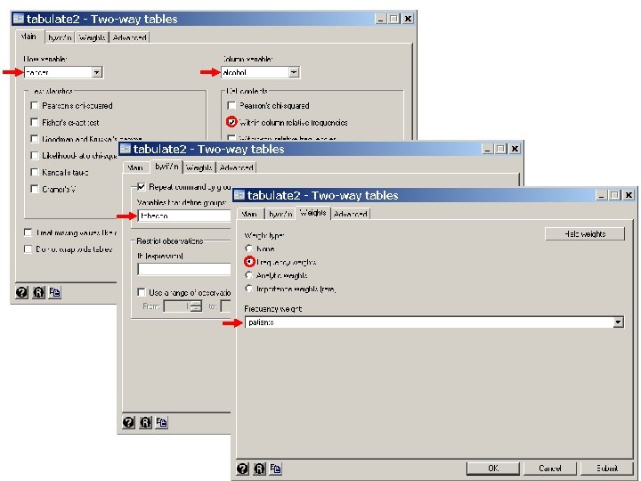
12. Example: Effect of Dose of Tobacco on Esophageal Cancer Risk . * 5. 12. Esophageal. Ca. Class. Version. do. *. * Estimate age-adjusted risk of esophageal cancer due to dose of tobacco. . *. use C: WDDtext5. 5. Esophageal. Ca. dta, clear. * Statistics > Summaries. . . > Tables > Two-way tables with measures. . tabulate cancer tobacco [freq=patients] , column +----------+ | Key | |----------| | frequency | | column percentage | +----------+ Esophageal | Tobacco (gm/day) Cancer | 0 -9 10 -19 20 -29 >= 30 | Total ------+----------------------+----- No | 447 178 99 51 | 775 | 85. 14 75. 42 75. 00 62. 20 | 79. 49 ------+----------------------+----- Yes | 78 58 33 31 | 200 | 14. 86 24. 58 25. 00 37. 80 | 20. 51 ------+----------------------+----- Total | 525 236 132 82 | 975 | 100. 00 | 100. 00

. * Statistics > Binary outcomes > Logistic regression (reporting odds ratios). logisitic cancer i. age i. tobacco [freq=patients] Logit regression No. of obs = 975 LR chi 2(8) = 157. 68 Prob > chi 2 = 0. 0000 Pseudo R 2 = 0. 1594 Log likelihood = -415. 90235 --------------------------------------- cancer | Odds Ratio Std. Err. z P>|z| [95% Conf. Interval] -------+-------------------------------- age | 2 | 6. 035932 6. 433686 1. 69 0. 092 . 7472235 48. 75713 3 | 36. 20831 37. 10835 3. 50 0. 000 4. 857896 269. 8785 4 | 61. 79318 63. 10432 4. 04 0. 000 8. 349838 457. 3019 5 | 83. 56952 85. 86437 4. 31 0. 000 11. 15506 626. 0713 6 | 60. 45383 64. 52449 3. 84 0. 000 7. 462882 489. 7124 | tobacco | 2 | 1. 835482 . 3781838 2. 95 0. 003 1. 225655 2. 748731 {1} 3 | 1. 945172 . 487733 2. 65 0. 008 1. 189947 3. 179717 4 | 5. 706139 1. 725688 5. 76 0. 000 3. 154398 10. 3221 --------------------------------------- {1} Note how similar the log-odds ratios for the 2 nd and 3 rd levels of tobacco exposure. If we had assigned a single parameter for tobacco we would have badly overestimated the odds ratio between levels 2 and 3, and badly underestimated the odds ratio between levels 1 and 2 and between levels 3 and 4.

. generate smoke = tobacco . * Data > Create. . . > Other variable-transformation. . . > Recode catigorical. . recode smoke 3=2 4=3 {2} (96 changes made) Syntax help {2} We want to combine the 2 nd and 3 rd levels of tobacco exposure. We do this by defining a new variable called smoke that is identical to tobacco and then using the recode statement, which in this example changes values of smoke = 3 to smoke = 2, and values of smoke = 4 to smoke = 3.

. label variable smoke "Smoking (gm/day)". label define smoke 1 "0 -9" 2 "10 -29" 3 ">= 30". label values smoke. * Statistics > Summaries. . . > Tables > Table of summary statistics (table). . table smoke tobacco [freq=patients], row col {3} ----------------------Smoking | Tobacco (gm/day) | 0 -9 10 -19 20 -29 >= 30 Total -----+----------------- 0 -9 | 525 525 10 -29 | 236 132 368 >= 30 | 82 82 | Total | 525 236 132 82 975 ----------------------- {3} This table statement shows that the previous recode statement worked.

. * Statistics > Binary outcomes > Logistic regression (reporting odds ratios). logistic cancer i. age i. smoke [freq=patients] Logistic regression Number of obs = 975 LR chi 2(7) = 157. 64 Prob > chi 2 = 0. 0000 Log likelihood = -415. 92589 Pseudo R 2 = 0. 1593 --------------------------------------- cancer | Odds Ratio Std. Err. z P>|z| [95% Conf. Interval] -------+-------------------------------- age | 2 | 6. 037092 6. 434914 1. 69 0. 092 . 7473691 48. 76637 3 | 36. 2117 37. 11182 3. 50 0. 000 4. 85835 269. 9038 4 | 61. 79965 63. 11096 4. 04 0. 000 8. 350705 457. 3503 5 | 83. 52177 85. 81492 4. 31 0. 000 11. 14879 625. 7078 6 | 60. 25337 64. 30389 3. 84 0. 000 7. 439742 487. 9831 | smoke | 2 | 1. 873669 . 3421356 3. 44 0. 001 1. 309972 2. 679933 {4} 3 | 5. 704954 1. 725242 5. 76 0. 000 3. 153836 10. 31965 ---------------------------------------. lincom 3. smoke - 2. smoke {5} ( 1) - [cancer]2. smoke + [cancer]3. smoke = 0 --------------------------------------- cancer | Odds Ratio Std. Err. z P>|z| [95% Conf. Interval] -------+-------------------------------- (1) | 3. 044803 . 9116935 3. 72 0. 000 1. 693118 5. 475593 ---------------------------------------

{4} There is a marked trend of increasing cancer risk with increasing dose of tobacco. Men who smoked 10 -29 grams a day had 1. 87 times the cancer risk of men who smoked less. Men who smoked more than 29 gm/day had 5. 7 times the cancer risk of men who smoked less than 10 grams a day. {5} The odds ratio for > 30 gm/day of tobacco relative to 10 -29 gm/day is 3. 04 and is highly significant. We do not need to check this box following the logistic command to exponentiate the linear sum of coefficients.

The next question is how do alcohol and tobacco interact on esophageal cancer risk? . * 5. 20. Esophageal. Ca. Class. Versionlog . * Regress esophageal cancers against age and dose of alcohol . * and tobacco using a multiplicative model. . * . use 5. 5. Esophageal. Ca. dta, clear . sort tobacco. * Statistics > Summaries. . . > Tables > Two-way tables with measures. . by tobacco: tabulate cancer alcohol [freq=patients] > , column {1} -> tobacco= 0 -9 Esophageal | Alcohol (gm/day) Cancer | 0 -39 40 -79 80 -119 >= 120 | Total ------+------------------+------- No | 252 145 42 8 | 447 | 96. 55 81. 01 68. 85 33. 33 | 85. 14 ------+------------------+------- Yes | 9 34 19 16 | 78 | 3. 45 18. 99 31. 15 66. 67 | 14. 86 ------+------------------+------- Total | 261 179 61 24 | 525 | 100. 00 | 100. 00 {1} by tobacco: produces separate frequency tables for each value of tobacco. The data set must first be sorted by tobacco.

-> tobacco= 10 -19 Esophageal | Alcohol (gm/day) Cancer | 0 -39 40 -79 80 -119 >= 120 | Total ------+------------------+------- No | 74 68 30 6 | 178 | 88. 10 80. 00 61. 22 33. 33 | 75. 42 ------+------------------+------- Yes | 10 17 19 12 | 58 | 11. 90 20. 00 38. 78 66. 67 | 24. 58 ------+------------------+------- Total | 84 85 49 18 | 236 | 100. 00 | 100. 00 -> tobacco= 20 -29 Esophageal | Alcohol (gm/day) Cancer | 0 -39 40 -79 80 -119 >= 120 | Total ------+------------------+------- No | 37 47 10 5 | 99 | 88. 10 75. 81 62. 50 41. 67 | 75. 00 ------+------------------+------- Yes | 5 15 6 7 | 33 | 11. 90 24. 19 37. 50 58. 33 | 25. 00 ------+------------------+------- Total | 42 62 16 12 | 132 | 100. 00 | 100. 00

-> tobacco= >= 30 Esophageal | Alcohol (gm/day) Cancer | 0 -39 40 -79 80 -119 >= 120 | Total ------+------------------+------- No | 23 20 5 3 | 51 | 82. 14 68. 97 41. 67 23. 08 | 62. 20 ------+------------------+------- Yes | 5 9 7 10 | 31 | 17. 86 31. 03 58. 33 76. 92 | 37. 80 ------+------------------+------- Total | 28 29 12 13 | 82 | 100. 00 | 100. 00 These tables show that the proportion of study subjects with cancer increases dramatically with increasing alcohol consumption for every level of tobacco consumption. The proportion of cases also increases with increasing tobacco consumption for most levels of alcohol.

13. Multiplicative Model of Effect of Smoking and Alcohol on Esophageal Cancer Risk Suppose that subjects either were or were not exposed to alcohol and tobacco and we did not include age in our model. Consider the model where mij is the number of subjects with drinking status i and smoking status j. dij is the number of cancers with drinking status i and smoking status j. , 1 and 2 are model parameters.

Thus the log-odds of a drinker with smoking status j is {4. 7} The log-odds of a non-drinker with smoking status j is Subtracting equation {4. 8} from {4. 7} gives that {4. 8} where ij is the probability that someone with drinking status i and smoking status j develops cancer. In other words, exp( 1) is the odds ratio for cancer in drinkers compared to non-drinkers adjusted for smoking. Note that this implies that the relative risk of drinking is the same in smokers and nonsmokers.

By an identical argument, exp( 2) is the odds ratio for cancer in smokers compared to non -smokers adjusted for drinking. For people who both drink and smoke the model is {4. 9} while for people who neither drink nor smoke the model is {4. 10} Subtracting {4. 9} from {4. 10} give that the log-odds ratio for people who both smoke and drink relative to those who do neither is 1 + 2, and the corresponding odds ratio is exp( 1) exp( 2). Thus our model implies that the odds ratio of having both risk factors equals the product of the individual odds ratio for drinking and smoking. It is for this reason that this is called a multiplicative model.

The multiplicative assumption is a very strong one that is often not justified. Let us see how it works with the Ille-et-Vilaine data set. . *. * Regress cancer against age, alcohol and smoke. . * Use a multiplicative model. *. * Statistics > Binary outcomes > Logistic regression (reporting odds ratios). logistic cancer i. age i. alcohol i. smoke [freq=patients] {1} Logistic regression Number of obs = 975 LR chi 2(10) = 285. 55 Prob > chi 2 = 0. 0000 Log likelihood = -351. 96823 Pseudo R 2 = 0. 2886 {1} This command fits a model with a constant parameter, 5 age parameters 3 alcohol parameters and two tobacco parameters. No parameter is given for the lowest strata associated with age, alcohol or smoke.

--------------------------------------- cancer | Odds Ratio Std. Err. z P>|z| [95% Conf. Interval] -------+-------------------------------- age | 2 | 7. 262526 8. 017757 1. 80 0. 073 . 834391 63. 21291 3 | 43. 65627 46. 62635 3. 54 0. 000 5. 381893 354. 1263 4 | 76. 3655 81. 33339 4. 07 0. 000 9. 469377 615. 8472 5 | 133. 7632 143. 9793 4. 55 0. 000 16. 22277 1102. 93 6 | 124. 4262 139. 5094 4. 30 0. 000 13. 82058 1120. 205 | alcohol | 2 | 4. 213304 1. 05191 5. 76 0. 000 2. 582905 6. 872854 {2} 3 | 7. 222005 2. 053957 6. 95 0. 000 4. 135936 12. 61077 4 | 36. 7912 14. 17012 9. 36 0. 000 17. 29434 78. 26794 | smoke | 2 | 1. 592701 . 3200884 2. 32 0. 021 1. 074154 2. 361577 3 | 5. 159309 1. 775207 4. 77 0. 000 2. 628521 10. 12679 --------------------------------------- {2} The odds ratio for level 2 drinkers relative to level 1 drinkers adjusted for age and smoking is 4. 21.

. lincom 2. alcohol + 2. smoke ( 1) [cancer]2. alcohol + [cancer]2. smoke = 0 --------------------------------------- cancer | Odds Ratio Std. Err. z P>|z| [95% Conf. Interval] -------+-------------------------------- (1) | 6. 710535 2. 110331 6. 05 0. 000 3. 623022 12. 4292 {3} ---------------------------------------. lincom 3. alcohol + 2. smoke ( 1) [cancer]3. alcohol + [cancer]2. smoke = 0 --------------------------------------- cancer | Odds Ratio Std. Err. z P>|z| [95% Conf. Interval] -------+-------------------------------- (1) | 11. 5025 3. 877641 7. 25 0. 000 5. 940747 22. 27118 ---------------------------------------. lincom 4. alcohol + 2. smoke ( 1) [cancer]4. alcohol + [cancer]2. smoke = 0 --------------------------------------- cancer | Odds Ratio Std. Err. z P>|z| [95% Conf. Interval] -------+-------------------------------- (1) | 58. 59739 25. 19568 9. 47 0. 000 25. 22777 136. 1061 ---------------------------------------

{3} The cancer log-odds for a man in, say, the third age strata who is a level 2 drinker and level 2 smoker is _cons + 3. age + 2. alcohol + 2. smoke The cancer log-odds for a man in the same age strata who is a level 1 drinker and level 1 smoker is _cons + 3. age Subtracting these two log-odds and exponentiating gives that the odds ratio for men who are both level 2 drinkers and level 2 smokers relative to those who are level 1 drinkers and level 1 smokers is 6. 71.

. lincom 2. alcohol + 3. smoke ( 1) [cancer]2. alcohol + [cancer]3. smoke = 0 --------------------------------------- cancer | Odds Ratio Std. Err. z P>|z| [95% Conf. Interval] -------+-------------------------------- (1) | 21. 73774 9. 508636 7. 04 0. 000 9. 223106 51. 23319 ---------------------------------------. lincom 3. alcohol + 3. smoke ( 1) [cancer]3. alcohol + [cancer]3. smoke = 0 --------------------------------------- cancer | Odds Ratio Std. Err. z P>|z| [95% Conf. Interval] -------+-------------------------------- (1) | 37. 26056 17. 06685 7. 90 0. 000 15. 18324 91. 43957 ---------------------------------------. lincom 4. alcohol + 3. smoke ( 1) [cancer]4. alcohol + [cancer]3. smoke = 0 --------------------------------------- cancer | Odds Ratio Std. Err. z P>|z| [95% Conf. Interval] -------+-------------------------------- (1) | 189. 8171 100. 9788 9. 86 0. 000 66. 91353 538. 4643 ---------------------------------------

The preceding analyses are summarized in the following table. Note that the multiplicative assumption holds. E. g. 36. 8 5. 16 = 190

Table 4. 1. Effect of Alcohol and Tobacco on Esophageal Cancer Risk Multiplicative Model -- Adjusted to Age Daily Tobacco Consumption Daily Alcohol Comsumption 0 -9 gm Odds Ratio 95% CI 10 -29 gm 30 gm Odds Ratio 95% CI 1. 59 (1. 1 - 2. 4) 5. 16 (2. 6 - 10) 0 -39 gm 1. 0* 40 -79 gm 4. 21 (2. 6 - 6. 9) 6. 71 (3. 6 - 12) 21. 7 (9. 2 - 51) 80 -119 gm 7. 22 (4. 1 - 13) 11. 5 (5. 9 - 22) 37. 3 (15 - 91) 120 gm. 36. 8 * Denominator of odds ratios (17 - 78) 58. 6 (25 - 140) 190 (67 - 540) This model suggests that combined heavy alcohol and tobacco consumption has an enormous effect on the risk of esophageal cancer. To determine if this is real or a model artifact we need to look at a model that permits the cancer risk associated with combined risk factors to deviate from the multiplicative model.

14. Modeling the Effect of Alcohol and Tobacco on Cancer Risk with Interaction Let us first return to the simple example where people either do or do not drink or smoke and where we do not adjust for age. Our multiplicative model was {4. 11} We allow alcohol and tobacco to have a synergistic effect on cancer odds by including a fourth parameter as follows {4. 12} Then 3 only enters the model for people who both smoke and drink. By the usual arguments…

1 is the log odds ratio for cancer associated with alcohol among non-smokers, 2 is the log odds ratio for cancer associated with smoking among non-drinkers, 1 + 3 is the log odds ratio for cancer associated with alcohol among smokers, 1 + 2 + 3 is the log odds ratio for cancer associated with people who smoke and drink compared to those who are both non-smokers and non-drinkers.

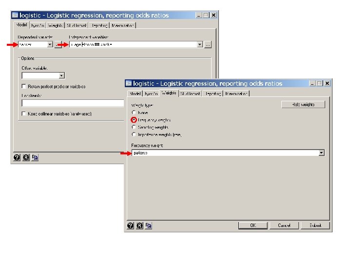
We now apply this interpretation to the esophageal cancer data. 5. 20. Esophagela. Class. Version. log continues as follows: . *. * Regress cancer against age, alcohol and smoke. . * Include alcohol-smoke interaction terms. . *. * Statistics > Binary outcomes > Logistic regression (reporting odds ratios). logistic cancer i. age alcohol##smoke [freq=patients], {1} Logistic regression Number of obs = 975 LR chi 2(16) = 290. 90 Prob > chi 2 = 0. 0000 Log likelihood = -349. 29335 Pseudo R 2 = 0. 2940

A separate parameter is fitted for each of these variables. In addition, the model specifies 5 parameters for the 5 age indicator variables and a constant parameter. {1} The syntax alcohol##smoke defines the following categorical values: 2. alcohol = 1 if alcohol = 2, and = 0 otherwise 3. alcohol = 1 if alcohol = 3, and = 0 otherwise 4. alcohol = 1 if alcohol = 4, and = 0 otherwise 2. smoke = 1 if smoke = 2, and = 0 otherwise 3. smoke = 1 if smoke = 3, and = 0 otherwise alcohol#smoke 2 2 = 2. alcohol x 2. smoke 2 3 = 2. alcohol x 3. smoke 3 2 = 3. alcohol x 2. smoke 3 3 = 3. alcohol x 3. smoke 4 2 = 4. alcohol x 2. smoke 4 3 = 4. alcohol x 3. smoke

--------------------------------------- cancer | Odds Ratio Std. Err. z P>|z| [95% Conf. Interval] -------+-------------------------------- age | 2 | 6. 697614 7. 41052 1. 72 0. 086 . 7657997 58. 57673 3 | 40. 1626 42. 67457 3. 48 0. 001 5. 004744 322. 3011 4 | 69. 55115 73. 73699 4. 00 0. 000 8. 707117 555. 5642 5 | 123. 0645 131. 6754 4. 50 0. 000 15. 11374 1002. 06 6 | 118. 8368 133. 2538 4. 26 0. 000 13. 19724 1070. 086 | alcohol | 2 | 7. 554406 3. 043769 5. 02 0. 000 3. 429574 16. 64028 3 | 12. 71358 5. 825002 5. 55 0. 000 5. 179306 31. 20788 4 | 65. 07188 39. 54145 6. 87 0. 000 19. 7767 214. 108 | smoke | 2 | 3. 800862 1. 703912 2. 98 0. 003 1. 578671 9. 151084 3 | 8. 651205 5. 569301 3. 35 0. 001 2. 449667 30. 55247 | alcohol#| smoke | 2 2 | . 3251915 . 1746668 -2. 09 0. 036 . 1134859 . 9318294 2 3 | . 5033299 . 4154539 -0. 83 0. 406 . 0998302 2. 53772 3 2 | . 3341452 . 2008274 -1. 82 0. 068 . 1028839 1. 085233 3 3 | . 657279 . 6598915 -0. 42 0. 676 . 0918681 4. 702563 4 2 | . 3731549 . 301804 -1. 22 0. 223 . 076462 1. 821095 4 3 | . 3489097 . 4210291 -0. 87 0. 383 . 032777 3. 714132 --------------------------------------- The highlighted odds ratios show age adjusted risks of drinking among level 1 smokers and smoking among level 1 drinkers

. lincom 2. alcohol + 2. smoke + 2. alcohol#2. smoke {2} ( 1) [cancer]2. alcohol + [cancer]2. smoke + [cancer]2. alcohol#2. smoke = 0 --------------------------------------- cancer | Odds Ratio Std. Err. z P>|z| [95% Conf. Interval] -------+-------------------------------- (1) | 9. 337306 3. 826162 5. 45 0. 000 4. 182379 20. 84586 --------------------------------------- {2} This statement calculates the odds ratio for men in the second strata of alcohol and smoke relative to men in the first strata of both of these variables. This odds ratio of 9. 33 is adjusted for age. 2. alcohol#2. smoke represents the parameter associated with the product of the covariates 2. alcohol and 2. smoke.

. lincom 2. alcohol + 3. smoke + 2. alcohol#3. smoke ( 1) [cancer]2. alcohol + [cancer]3. smoke + [cancer]2. alcohol#3. smoke = 0 --------------------------------------- cancer | Odds Ratio Std. Err. z P>|z| [95% Conf. Interval] -------+-------------------------------- (1) | 32. 89498 19. 73769 5. 82 0. 000 10. 14824 106. 6274 ---------------------------------------. lincom 3. alcohol + 2. smoke + 3. alcohol#2. smoke ( 1) [cancer]3. alcohol + [cancer]2. smoke + [cancer]3. alcohol#2. smoke = 0 --------------------------------------- cancer | Odds Ratio Std. Err. z P>|z| [95% Conf. Interval] -------+-------------------------------- (1) | 16. 14675 7. 152595 6. 28 0. 000 6. 776802 38. 47207 ---------------------------------------

. lincom 3. alcohol + 3. smoke + 3. alcohol#3. smoke ( 1) [cancer]3. alcohol + [cancer]3. smoke + [cancer]3. alcohol#3. smoke = 0 --------------------------------------- cancer | Odds Ratio Std. Err. z P>|z| [95% Conf. Interval] -------+-------------------------------- (1) | 72. 29267 57. 80896 5. 35 0. 000 15. 08098 346. 5446 ---------------------------------------. lincom 4. alcohol + 2. smoke + 4. alcohol#2. smoke ( 1) [cancer]4. alcohol + [cancer]2. smoke + [cancer]4. alcohol#2. smoke = 0 --------------------------------------- cancer | Odds Ratio Std. Err. z P>|z| [95% Conf. Interval] -------+-------------------------------- (1) | 92. 29212 53. 97508 7. 74 0. 000 29. 33307 290. 3833 ---------------------------------------. lincom 4. alcohol + 3. smoke + 4. alcohol#3. smoke ( 1) [cancer]4. alcohol + [cancer]3. smoke + [cancer]4. alcohol#3. smoke = 0 --------------------------------------- cancer | Odds Ratio Std. Err. z P>|z| [95% Conf. Interval] -------+-------------------------------- (1) | 196. 4188 189. 1684 5. 48 0. 000 29. 74417 1297. 072 ---------------------------------------

The following table summarizes the results of this analysis

Table 4. 2. Effect of Alcohol and Tobacco on Esophageal Cancer Risk Model with all 2 -Way Interaction Terms -- Adjusted for Age Tables 4. 1 and 4. 2 are quite consistent, and both indicate a dramatic increase in risk with increased drinking and smoking. Note that the confidence intervals are wide, particularly for the most heavily exposed subjects. The confidence intervals are wider in Table 4. 2 because they are derived from a model with more parameters. Which model is better?

Table 4. 1. Effect of Alcohol and Tobacco on Esophageal Cancer Risk Multiplicative Model -- Adjusted to Age Daily Tobacco Consumption Daily Alcohol Comsumption 0 -9 gm Odds Ratio 95% CI 10 -29 gm 30 gm Odds Ratio 95% CI 1. 59 (1. 1 - 2. 4) 5. 16 (2. 6 - 10) 0 -39 gm 1. 0* 40 -79 gm 4. 21 (2. 6 - 6. 9) 6. 71 (3. 6 - 12) 21. 7 (9. 2 - 51) 80 -119 gm 7. 22 (4. 1 - 13) 11. 5 (5. 9 - 22) 37. 3 (15 - 91) 120 gm. 36. 8 * Denominator of odds ratios (17 - 78) 58. 6 (25 - 140) 190 (67 - 540)

15. Model Fitting: Nested Models and Model Deviance A model is said to be nested within a second model if the first model is a special case of the second. For example, the multiplicative model {4. 11} discussed before was while model {4. 12} contained an interaction term and was Model {4. 11} is nested within model {4. 12} since model {4. 11} is a special case of model {4. 12} with 3 = 0.

The model Deviance D is a statistic derived from the likelihood function that measures goodness of fit of the data to a specific model. Let log(L) denote the maximum value of the log likelihood function. Then the deviance is given by D = K – 2 log(L) {4. 13} for some constant K that is independent of the model parameters. If the model is correct then for large sample sizes D has a 2 distribution with degrees of freedom equal to the number of observations minus the number of parameters. Regardless of the true model, D is a non-negative number. Large values of D indicate poor model fit; a perfect fit has D = 0.

Suppose that D 1 and D 2 are deviances from two models with model 1 nested in model 2. Then it can be shown that if model 1 is true then = D 1 – D 2 has an approximately 2 distribution with the number of degrees of freedom equal to the number of parameters in model 2 minus the number of parameters in model 1. Equivalently, = D 1 – D 2 = We use the reduction in deviance as a guide to building reasonable models for our data.

For example, in the multiplicative model of alcohol and tobacco levels analyzed above the log likelihood was log(L) = -351. 96823 . * Statistics > Binary outcomes > Logistic regression (reporting odds ratios). logistic cancer i. age i. alcohol i. smoke [freq=patients] Logistic regression Number of obs = 975 LR chi 2(10) = 285. 55 Prob > chi 2 = 0. 0000 Log likelihood = -351. 96823 Pseudo R 2 = 0. 2886 The corresponding model with the 6 interaction terms has a log likelihood of log(L) = -349. 29335 . * Statistics > Binary outcomes > Logistic regression (reporting odds ratios). logistic cancer i. age alcohol##smoke [freq=patients], Logistic regression Number of obs = 975 LR chi 2(16) = 290. 90 Prob > chi 2 = 0. 0000 Log likelihood = -349. 29335 Pseudo R 2 = 0. 2940

For example, in the multiplicative model of alcohol and tobacco levels analyzed above the log likelihood was log(L 1) = -351. 96823 The corresponding model with the 6 interaction terms has a log likelihood of log(L 2) = -349. 29335 = 2(-349. 29335 + 351. 96823) = 5. 35

Since there are 6 more parameters in the interactive model than the multiplicative model, has a 2 distribution with 6 degrees of freedom under the independent model. We calculate the P value in Stata with the command display chi 2 tail(6, 5. 34976) which gives P =. 50. Thus there is no statistical evidence to suggest that the multiplicative model is false, or that any meaningful improvement in the model fit can be obtained by adding interaction terms to the model. So what results should we publish – Table 4. 1 or 4. 2?

In general, I am guided by deviance reduction statistics when deciding whether to include variables that may, or may not be true confounders, but that are not intrinsically of interest. If I am interested in the joint effects of 2 or more variables, I usually include the interaction term unless the inclusion of the interaction parameter has almost no effect on the resulting relative risk estimates. There are no hard and fast guidelines to model building other than that it is best not to include uninteresting variables in the model that have a trivial effect on the model deviance. I think I personally would go with Table 4. 2 over 4. 1 in spite of the lack of evidence of interaction. The odds ratio for both >120 gm alcohol and >30 gm tobacco is so large that I would worry that we were being misled by not taking into account a small but real interaction term. It would also be acceptable to say that we analyzed the data both ways, found no evidence of interaction, got comparable results and were presenting the multiplicative model results only.

Table 4. 1. Effect of Alcohol and Tobacco on Esophageal Cancer Risk Multiplicative Model -- Adjusted to Age Daily Tobacco Consumption Daily Alcohol Comsumption 0 -9 gm Odds Ratio 95% CI 10 -29 gm 30 gm Odds Ratio 95% CI 1. 59 (1. 1 - 2. 4) 5. 16 (2. 6 - 10) 0 -39 gm 1. 0* 40 -79 gm 4. 21 (2. 6 - 6. 9) 6. 71 (3. 6 - 12) 21. 7 (9. 2 - 51) 80 -119 gm 7. 22 (4. 1 - 13) 11. 5 (5. 9 - 22) 37. 3 (15 - 91) 120 gm. 36. 8 * Denominator of odds ratios (17 - 78) 58. 6 (25 - 140) 190 (67 - 540)

Table 4. 2. Effect of Alcohol and Tobacco on Esophageal Cancer Risk Model with all 2 -Way Interaction Terms -- Adjusted for Age

16. Influence Analysis for Logistic Regression Consider a logistic regression model with J distinct covariate patterns dj events occur among nj patients with the covariate pattern xj 1, xj 2, …xjq. Let j = denote the probability that a patient with the jth pattern of covariate values suffers an event. Then dj has a binomial distribution with expected value nj j standard error Hence will have a mean of 0 and a standard error of 1.

Let be the estimate of j obtained by substituting the maximum likelihood parameter estimates into the logistic probability function. Then the residual for the jth covariate pattern is The Pearson residual is which should have a mean of 0 and a standard deviation of 1 if the model is correct and if is a good estimate of the standard error of . The leverage hj is analogous to leverage in linear regression. It measures to potential of a covariate pattern to influence our parameter estimates if the associated residual is large.

For our purposes we can define hj by the formula In other words, 100(1 -hj) is the percent reduction in the variance of the jth residual due to the fact that the estimate of is pulled towards dj. The value of hj lies between 0 and 1. When hj is very small dj has almost no effect on its estimated expected value . When hj is close to 1, then . This implies that both the residual and its variance will be close to zero.

The standardized Pearson residual for the jth covariate pattern is the residual divided by its standard error. That is, This residual is analogous to the studentized residual for linear regression. rsj small. has mean 0 and standard error 1 is not necessarily normally distributed when nj is The square of the standardized Pearson residual is denoted We will use the critical value as a very rough guide to identifying large values of . Approximately 95% of these squared residuals should be less than 3. 84 if the logistic regression model is correct.

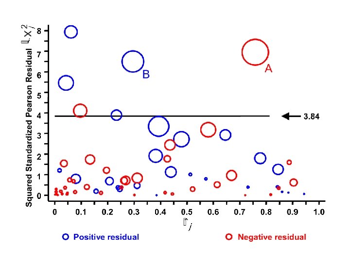
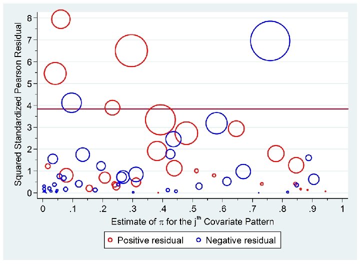
The influence statistic is a measure of the influence of the jth covariate pattern on all of the parameter estimates taken together. It equals Note that increases with both the magnitude of the standardized residual and the size of the leverage. It is analogous to Cook’s distance for linear regression. Covariate patterns associated with large values of and merit special attention. The following plot is for our model of alcohol and tobacco dose with interaction terms and plots against The area of the circles is proportional to

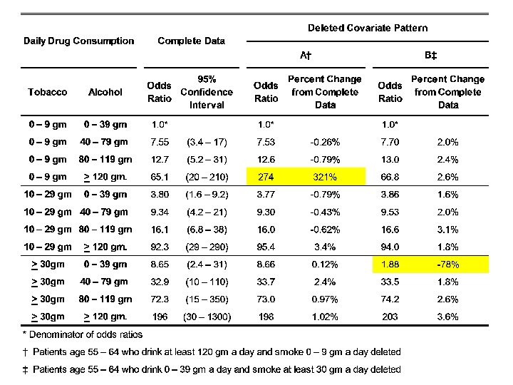
There are 68 unique covariate patterns in this data set. 5% of 68 equals 3. 4 There are 6 residuals greater than 3. 84. There are 2 large squared residuals with high influence. Residual A is associated with patients who are age 55 – 64 and consume, on a daily basis, at least 120 gm of alcohol 0 – 9 gm of tobacco. Residual B is associated with patients who are age 55 – 64 and consume, on a daily basis, 0 – 39 gm of alcohol and at least 30 gm of tobacco. The influence statistics associated with residuals A and B are 6. 16 and 4. 15, respectively.

NOTE: In linear regression observations with high influence are due to a single patient and we have the option of deleting the patient In logistic regression covariate patters with high influence indicate poor model fit. However, we usually do not have the option of deleting the pattern if it represents a sizable number of patients.

Table 4. 1. Effect of Alcohol and Tobacco on Esophageal Cancer Risk Daily Tobacco Consumption Daily Alcohol Comsumption 0 -9 gm Odds Ratio 95% CI 10 -29 gm 30 gm Odds Ratio 95% CI 1. 59 (1. 1 - 2. 4) 5. 16 (2. 6 - 10) Multiplicative Model -- Adjusted to Age 0 -39 gm 1. 0* 40 -79 gm 4. 21 (2. 6 - 6. 9) 6. 71 (3. 6 - 12) 21. 7 (9. 2 - 51) 80 -119 gm 7. 22 (4. 1 - 13) 11. 5 (5. 9 - 22) 37. 3 (15 - 91) 120 gm. 36. 8 (17 - 78) 58. 6 (25 - 140) 190 (67 - 540) Model with all 2 -Way Interaction Terms -- Adjusted for Age 0 – 39 gm 1. 0* 40 – 79 gm 7. 55 80 – 119 gm >120 gm 3. 8 (1. 6 – 9. 2) 8. 65 (2. 4 – 31) (3. 4 – 17) 9. 34 (4. 2 – 21) 32. 9 (10 – 110) 12. 7 (5. 2 – 31) 16. 1 (6. 8 – 38) 72. 3 (15 – 350) 65. 1 (20 – 210) 92. 3 (29 – 290) 196 (30 – 1300) * Denominator of odds ratios

17. What is the best model? We have 975 patients, 200 cases, 68 unique covariate patterns 17 parameters in the interactive model. Over-fitting is certainly a concern Still the effect of dose of tobacco and alcohol on risk is very marked, which makes the interactive model tempting to use. It is a pity that age, alcohol and tobacco were categorized before we received this data. It is always a mistake to throw such data away. If we had the continuous data we could fit a cubic spline model with 1 constant parameter 6 spline parameters: 2 each for age alcohol and tobacco 4 interaction parameters for a total of 11 parameters, which would be more reasonable.

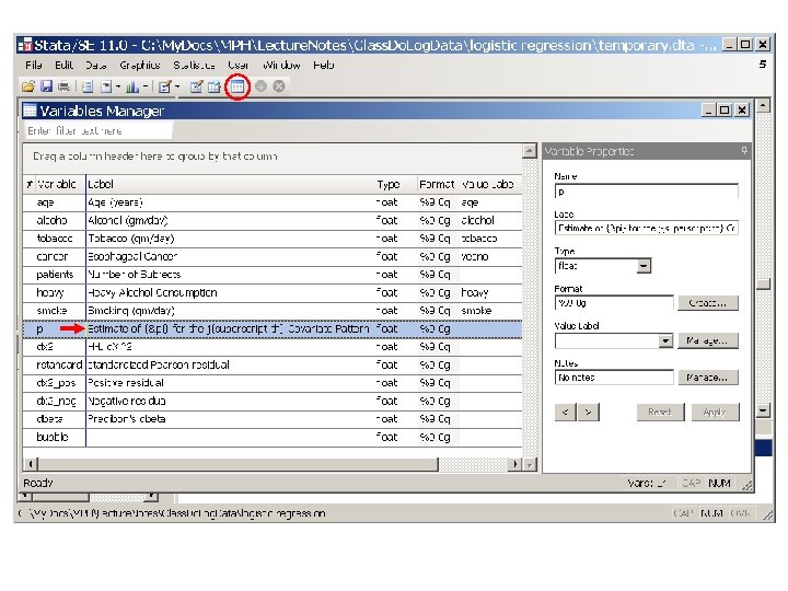
18. Residual analysis with Stata 5. 20. Esophagela. Class. Version. log continues as follows. *. * Perform residual analysis. *. * Statistics > Postestimation > Predictions, residuals, etc. . predict p, p {1} The p option in this predict command defines the variable p to equal . In this and the next two predict commands the name of the newly defined variable is the same as the command option. {1}

. predict dx 2, dx 2 (57 missing values generated) {2} Define the variable dx 2 to equal . All records with the same covariate pattern are given the same value of dx 2. {2}

. predict rstandard, rstandard (57 missing values generated) {3} Define rstandard to equal the standardized Pearson residual . {3}

. generate dx 2_pos = dx 2 if rstandard >= 0 (137 missing values generated) . generate dx 2_neg = dx 2 if rstandard < 0 (112 missing values generated) {4} . label variable dx 2_pos "Positive residual". label variable dx 2_neg "Negative residual". label variable p /// "Estimate of {&pi} for the j{superscript: th} Covariate Pattern" {5} {4} We are going to draw a scatterplot of against . We would like to color code the plotting symbols to indicate if the residual is positive or negative. This command defines dx 2_pos to equal if and only if is non-negative. The next command defines dx 2_neg to equal if is negative. {5} Greek lettters, superscripts, italics, etc can be entered in variable labels. {&pi} enters the letter into the label. {superscript: th} writes the letters “th” as a superscript.

. predict dbeta, dbeta {5} (57 missing values generated) {5} Define the variable dbeta to equal . The values of dx 2, dbeta and rstandard are affected by the number of subjects with a given covariate pattern, and the number of events that occur to these subjects. They are not affected by the number of records used to record this information. Hence, it makes no difference whethere is one record per patient or just two records specifying the number of subjects with the specified covariate pattern who did, or did not, suffer the event of interest.

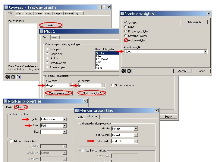
. scatter dx 2_pos p [weight=dbeta] /// {6} > , msymbol(Oh) mlwidth(medthick) mcolor(red) /// {7} > || scatter dx 2_neg p [weight=dbeta] /// > , msymbol(Oh) mlwidth(medthick) mcolor(blue) /// > ||, ylabel(0(1)8, angle(0)) /// > ymtick(0(. 5)8) yline(3. 84, lwidth(medthick)) /// > xlabel(0(. 1)1) xmtick(0(. 05)1) /// > ytitle("Squared Standardized Pearson Residual") xscale(titlegap(2)) (analytic weights assumed) {6} This graph produces a scatterplot of against that is shown in the next slide. The [weight=dbeta] command modifier causes the plotting symbols to be circles whose area is proportional to the variable dbeta. We plot both dx 2_pos and dx 2_neg against p in order to be able to assign different colors to values of that are associated with positive or negative residuals. {7} mlwidth defines the width of the marker lines. This is, the width of the circles. mcolor defines the marker color.

Red bubbles

Red Blue bubbles

Red Blue bubbles

19. Restricted Cubic Splines and Logistic Regression In the following example we use restricted cubic splines to model the effect of baseline MAP on hospital mortality in the SUPPORT data set. . * SUPPORTlogistic. RCS. log. *. * Regress mortal status at discharge against MAP . * in the SUPPORT data set (Knaus et al. 1995). . *. use "C: WDDtext3. 25. 2. SUPPORT. dta" , replace. *. * Calculate the proportion of patients who die in hospital. * stratified by MAP. . *. generate map_gr = round(map, 5). sort map_gr {1} . label variable map_gr "Mean Arterial Pressure (mm Hg)". * Data > Create or change data > Create new variable (extended). by map_gr: egen proportion = mean(fate) {2}

{1} round(map, 5) rounds map to the nearest integer divisible by 5. {2} This command defines proportion to equal the average value of fate over all records with the same value of map_gr. Since fate is a zero-one indicator variable, proportion will be equal to the proportion of patients with the same value of map_gr who die (have fate = 1). This command requires that the data set be sorted by the by variable (map_gr).

. generate = 100*proportion. label variable rate "Observed In-Hospital Mortality Rate (%)". generate deaths = map_gr if fate (747 missing values generated)

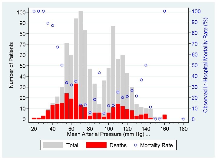
. *. * Draw an exploratory graph showing the number of patients, . * the number of deaths and the mortality rate for each MAP. . *. twoway histogram map_gr, discrete frequency color(gs 13) gap(20) /// {3} > || histogram deaths, discrete frequency color(red) gap(20) /// {4} > || scatter rate map_gr, yaxis(2) symbol(Oh) color(blue) /// > , xlabel(20 (20) 180) ylabel(0(10)100, angle(0)) /// > xmtick(25 (5) 175) ytitle(Number of Patients) /// > ylabel(0 (10) 100, angle(0) labcolor(blue) axis(2)) /// > ytitle(, color(blue) axis(2)) /// > legend(order(1 "Total" 2 "Deaths" 3 "Mortality Rate" ) /// > rows(1)) {3} The command twoway histogram map_gr produces a histogram of the variable map_gr. The discrete option specifies that a bar is to be drawn for each distinct value of map_gr; frequency specifies that the y-axis will be the number of patients at each value of map_gr; color(gs 13) specifies that the bars are to be light gray and gap(20) reduces the bar width by 20% to provide separation between adjacent bars. {4} This line of this command overlays a histogram of the number of in-hospital deaths on the histogram of the total number of patients.

These dialogue boxes show to create the gray histogram on the next slide. The dialog boxes for the red histogram are similar. Dialogue boxes for the scatter plot, axes and legends have been given previously.

. *. * Regress in-hospital mortality against MAP using simple . * logistic regression. . *. * Statistics > Binary outcomes > Logistic regression (reporting odds ratios). logistic fate map {5} Logistic regression Number of obs = 996 LR chi 2(1) = 29. 66 Prob > chi 2 = 0. 0000 Log likelihood = -545. 25721 Pseudo R 2 = 0. 0265 --------------------------------------- fate | Odds Ratio Std. Err. z P>|z| [95% Conf. Interval] -------+-------------------------------- map | . 9845924 . 0028997 -5. 27 0. 000 . 9789254 . 9902922 ---------------------------------------. * Statistics > Postestimation > Manage estimation results > Store in memory. estimates store simple {6} {5} This command regresses fate against map using simple logistic regression. {6} This command stores parameter estimates and other statistics from the most recent regression command. These statistics are stored under the name simple. We will use this information later to calculate the change in model deviance.

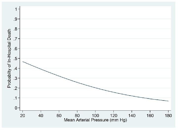
. predict p, p {7} . label variable p "Probabilty of In-Hospital Death". line p map, ylabel(0(. 1)1, angle(0)) xlabel(20(20)180) {7} The p option of this predict command defines p equal to the predicted probability of in-hospital death under the model. That is

. * Variables Manager. drop p. *. * Repeat the preceding model using restricted cubic splines . * with 5 knots at their default locations. . *. * Data > Create. . . > Other variable-creation. . . > linear and cubic. . mkspline _Smap = map, cubic displayknots | knot 1 knot 2 knot 3 knot 4 knot 5 -------+--------------------------- map | 47 66 78 106 129 . * Statistics > Binary outcomes > Logistic regression (reporting odds ratios). logistic fate _S* {8} Logistic regression Number of obs = 996 LR chi 2(4) = 122. 86 {9} Prob > chi 2 = 0. 0000 Log likelihood = -498. 65571 Pseudo R 2 = 0. 1097 --------------------------------------- fate | Odds Ratio Std. Err. z P>|z| [95% Conf. Interval] -------+-------------------------------- _Smap 1 | . 8998261 . 0182859 -5. 19 0. 000 . 8646907 . 9363892 _Smap 2 | 1. 17328 . 2013998 0. 93 0. 352 . 838086 1. 642537 _Smap 3 | 1. 0781 . 7263371 0. 11 0. 911 . 2878645 4. 037664 _Smap 4 | . 6236851 . 4083056 -0. 72 0. 471 . 1728672 2. 250185 ---------------------------------------

{8} Regress fate against MAP using a 5 -knot RCS logistic regression model. {9} Testing the null hypothesis that mortality is unrelated to MAP under this model is equivalent to testing the null hypothesis that all of the parameters associated with the spline covariates are zero. The likelihood ratio χ2 statistic to test this hypothesis equals 122. 86. It has four degrees of freedom and is highly significant P < 0. 00005.

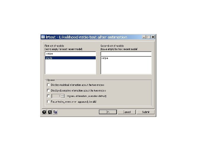
. *. * Test null hypotheses that the logit of the probability of. * in-hospital death is a linear function of MAP. . *. * Statistics > Postestimation > Tests > Likelihood-ratio test. lrtest simple. {10} Likelihood-ratio test LR chi 2(3) = 93. 20 (Assumption: simple nested in. ) Prob > chi 2 = 0. 0000 {10} This lrtest command calculates the likelihood ratio test of the null hypothesis that there is a linear relationship between the log odds of in-hospital death and baseline MAP. This is equivalent to testing the null hypothesis that _Smap 2 = _Smap 3 = _Smap 4 = 0. The lrtest command calculates the change in model deviance between two nested models. In this command, simple is the name of the model output saved by the previous estimates store command (see Comment 6). The period (. ) refers to the estimates from the most recently executed regression command. The user must insure that the two models specified by this command are nested. The change in model deviance equals 93. 2. Under the null hypothesis that the simple logistic regression model is correct this statistic will have an approximately chi-squared distribution with three degrees of freedom. The P value associated with this statistic is (much) less than 0. 00005.

. display 2*(545. 25721 -498. 65571) 93. 203 {11} Here we calculate the change in model deviance by hand from the maximum values of the log likelihood functions of the two models under consideration. Note that this gives the same answer as the preceding lrtest command. N. B. We can always test the validity of a simple logistic regression model by running a RCS model with k knots and then testing the null hypothesis of whether the second through k-1 th spline covariate parameters are simultaneously zero. In other words, we test the null hypothesis that the simple logisitic regression model is valid by testing the null hypothesis that the second through k-1 th spline covariate parameters are simultaneously zero. If we run a three-knot model then testing whether the second spline covariate parameter is zero is equivalent to testing the validity of the simple logistic regression model.

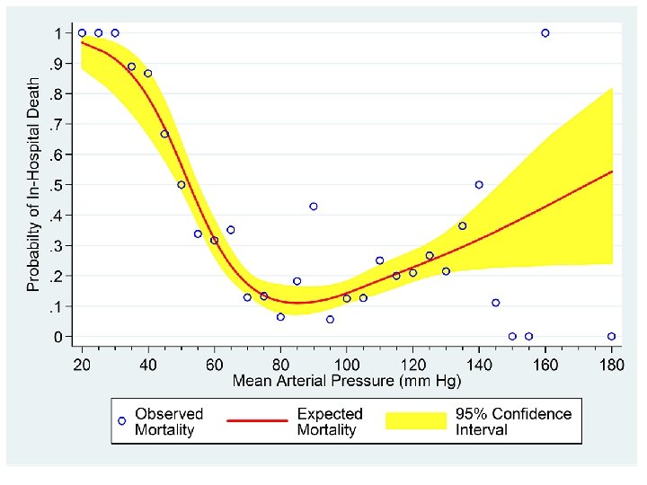
. *. * Plot the estimated probability of death against MAP together . * with the 95% confidence interval for this curve. Overlay . * the MAP-specific observed mortality rates. . *. predict p, p {12} . predict logodds, xb. predict stderr, stdp. generate p 2 = exp(logodds)/(1+exp(logodds)). *. * The values of p and p 2 are identical. . *. scatter p p 2 {12} The variable p is the estimated probability of in-hospital death from model our 5 knot RCS model.

p and p 2 equal the estimated probability of inhospital death. If we had used the glm command we would have needed to calculate p 2 directly since the p option is not available following glm.

. generate lodds_lb = logodds - 1. 96*stderr. generate lodds_ub = logodds + 1. 96*stderr. generate ub_p = exp(lodds_ub)/(1+exp(lodds_ub)) {13} . generate lb_p = exp(lodds_lb)/(1+exp(lodds_lb)). twoway rarea lb_p ub_p map, color(yellow) /// > || line p map, lwidth(medthick) color(red) /// > || scatter proportion map_gr, symbol(Oh) color(blue) /// > , ylabel(0(. 1)1, angle(0)) xlabel(20 (20) 180) /// > xmtick(25(5)175) ytitle(Probabilty of In-Hospital Death) /// > legend(order(3 "Observed" "Mortality" 2 "Expected" "Mortality" /// > 1 "95% Confidence" "Interval") rows(1)) {13} The variables lb_p and ub_p are the lower and upper 95% confidence bounds for p, respectively.

. *. * Determine the spline covariates at MAP = 90. *. list _S* if map == 90 {14} +---------------------+ | _Smap 1 _Smap 2 _Smap 3 _Smap 4 | |---------------------| 575. | 90 11. 82436 2. 055919 . 2569899 | {output omitted} 581. | 90 11. 82436 2. 055919 . 2569899 | +---------------------+. *. * Let or 1 = _Smap 1 minus the value of _Smap 1 at 90. . * Define or 2, or 3 and or 3 in a similar fashion. . *. generate or 1 = _Smap 1 - 90. generate or 2 = _Smap 2 - 11. 82436 . generate or 3 = _Smap 3 - 2. 055919. generate or 4 = _Smap 4 - . 2569899

{14} List the values of the spline covariates for the seven patients in the data set with a baseline MAP of 90. Only one or these identical lines of output are shown here. N. B. logodds[map] = logodds[90] = logodds[map] - logodds[90] = exp[logodds[map] - logodds[90] ] = odds ratio of a patient with MAP = map compared to a patient with a MAP = 90 by the usual argument.

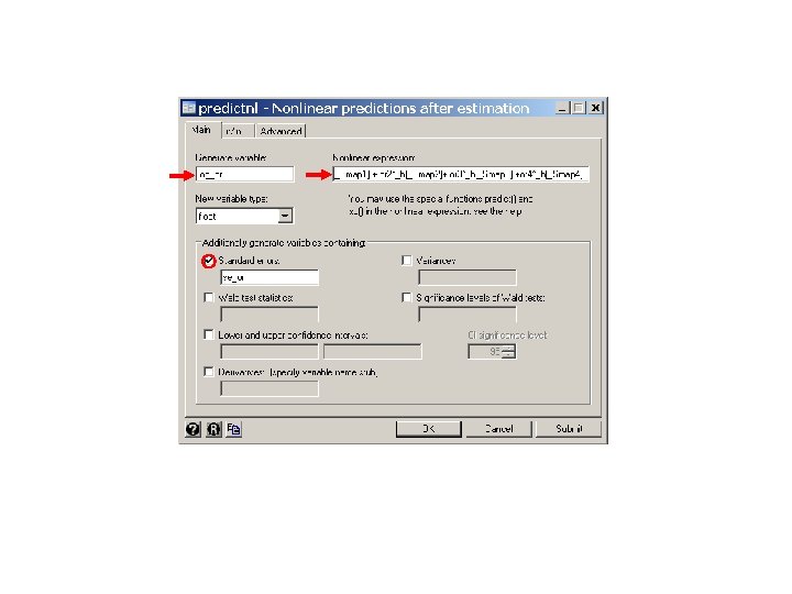
. *. * Calculate the log odds ratio for in-hospital death . * relative to patients with MAP = 90. . *. * Statistics > Postestimation > Nonlinear predictions. predictnl log_or = or 1*_b[_Smap 1] + or 2*_b[_Smap 2] /// > + or 3*_b[_Smap 3] +or 4*_b[_Smap 4], se(se_or) {16} {15} Define log_or to be the mortal log odds ratio for the ith patient in comparison to patients with a MAP of 90. The parameter estimates from the most recent regression command may be used in generate commands and are named _b[varname]. For example, in this RCS model _b[_Smap 2] = = 1. 17328; or 2 = _Smap 2 - 11. 82436. The command predictnl may be used to estimate non-linear functions of the parameter estimates. It is also very useful for calculating linear combinations of these estimates as is illustrated here. {16} The option se(se_or) calculates a new variable called se_or which equals the standard error of the log odds ratio.

. generate lb_log_or = log_or - 1. 96*se_or. generate ub_log_or = log_or + 1. 96*se_or. generate or = exp(log_or) {17} . generate lb_or = exp(lb_log_or) {18} . generate ub_or = exp(ub_log_or) {17} The variable or equals the odds ratio for in-hospital death for each patient relative to that for a patient with MAP = 90. {18} The variables lb_or and ub_or equal the lower and upper bounds of the 95% confidence interval for this odds ratio

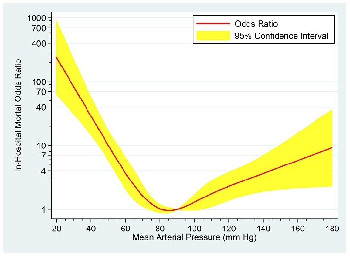
. . twoway rarea lb_or ub_or map, color(yellow) /// > || line or map, lwidth(medthick) color(red) /// > , ylabel(1 (3) 10 40(30)100 400(300)1000, angle(0)) /// > ymtick(2(1)10 20(10)100 200(100)900) yscale(log) /// {19} > xlabel(20 (20) 180) xmtick(25 (5) 175) /// > ytitle(In-Hospital Mortal Odds Ratio) /// > legend(ring(0) position(2) order(2 "Odds Ratio" /// > 1 "95% Confidence Interval") cols(1)) {19} yscale(log) plots the y-axis on a logarithmic scale.

These dialogue boxes illustrate how to select a lograthmic scale for the y-axis

20. Frequency Matched Case-Control Studies We often have access to many more potential control patients than case patients for case-control studies. If the distribution of some important confounding variable, such as age, differs markedly between cases and control, we may wish to adjust for this variable when designing the study. One way to do this is through frequency matching. The cases and potential controls are stratified into a number of groups based on, say, age. We then randomly select from each stratum the same number of controls as there are cases in the stratum. The data can then be analyzed by logistic regression with a classification variable to indicate the strata (see the analysis of the esophageal cancer and alcohol data in this chapter, Section 5 and 6). It is important, however, to keep the strata fairly large if logistic regression is to be used for the analysis. Otherwise the estimates of the parameters of real interest may be seriously biased. Breslow and Day (Vol. I, p. 251 -253) recommend that the strata be large enough so that each stratum contains at least 10 cases and 10 control. Even strata this large can lead to appreciable bias if the odds ratio being estimated is greater then 2.

a) Conditional logistic regression analysis Sometimes there are more than one important confounders that we would like to adjust for in the design of our study. In this case, we typically match each case patient to one or more controls with the same values of the confounding variables. This approach is often quite reasonable. However, it usually leads to strata (matched pairs or sets of patients) that are too small to be analyzed accurately with logistic regression. In this case, an alternate technique called conditional logistic regression should be used. This technique is discussed in Breslow and Day, Vol. I. In Stata, the clogit command may be used to implement these analyses.

21. What we have covered v Extend simple logistic regression to models with multiple covariates v Similarity between multiple linear and multiple logistic regression logit v Multiple 2 x 2 tables and the Mantel-Haenszel test Ø Estimating an odds ratio that is adjusted for a confounding variable v Using logistic regression as an alternative to the Mantel-Haenszel test v Using indicator covariates to model categorical variables i. varname notation in Stata ib#. varname notation in Stata v Making inferences about odds ratios derived from multiple parameters The Stata lincom command v Analyzing complex data with logistic regression Ø Multiplicative models Ø Models with interaction v Assessing model fit Ø Testing the change in model deviance in nested models Ø Evaluating residuals and influence v Using restricted cubic splines in logistic regression models Ø Plotting the probability of an outcome with confidence bands Ø Plotting odds ratios and confidence bands The Stata predictnl command

Cited References Breslow, N. E. and N. E. Day (1980). Statistical Methods in Cancer Research: Vol. 1 - The Analysis of Case-Control Studies. Lyon, France, IARC Scientific Publications. Knaus, W. A. , Harrell, F. E. , Jr. , Lynn, J. , Goldman, L. , Phillips, R. S. , Connors, A. F. , Jr. et al. The SUPPORT prognostic model. Objective estimates of survival for seriously ill hospitalized adults. Study to understand prognoses and preferences for outcomes and risks of treatments. Ann Intern Med. 1995; 122: 191 -203. Tuyns, A. J. , G. Pequignot, et al. (1977). Le cancer de L'oesophage en Ille-et-Vilaine en fonction des niveau de consommation d'alcool et de tabac. Des risques qui se multiplient. Bull Cancer 64: 45 -60. For additional references on these notes see. Dupont WD. Statistical Modeling for Biomedical Researchers: A Simple Introduction to the Analysis of Complex Data. 2 nd ed. Cambridge, U. K. : Cambridge University Press; 2009.