Iterative Program Analysis Abstract Interpretation Mooly Sagiv http

Iterative Program Analysis Abstract Interpretation Mooly Sagiv http: //www. cs. tau. ac. il/~msagiv/courses/pa 12 -13. html Tel Aviv University 640 -6706 Textbook: Principles of Program Analysis Chapter 4 CC 79, CC 92 1
![Specialized Chaotic Iterations System of Equations S= dfentry[s] = dfentry[v] = {f(u, v) (dfentry[u])](http://slidetodoc.com/presentation_image_h/a6533b7be3a34d45f0a55be12528e9a1/image-2.jpg "Specialized Chaotic Iterations System of Equations S= dfentry[s] = dfentry[v] = {f(u, v) (dfentry[u])")
Specialized Chaotic Iterations System of Equations S= dfentry[s] = dfentry[v] = {f(u, v) (dfentry[u]) | (u, v) E } FS: Ln Ln FS (X)[s] = FS(X)[v] = {f(u, v)(X[u]) | (u, v) E } lfp(S) = lfp(FS)
: Graph, s: Node, L: Lattice, : L, f: E")
Specialized Chaotic Iterations Chaotic(G(V, E): Graph, s: Node, L: Lattice, : L, f: E (L L) ){ for each v in V to n do dfentry[v] : = df[s] = WL = {s} while (WL ) do select and remove an element u WL for each v, such that. (u, v) E do temp = f(e)(dfentry[u]) new : = dfentry(v) temp if (new dfentry[v]) then dfentry[v] : = new; WL : = WL {v}
![WL [x 0, y 0, z 0] 1 {1} z =3 e. e[z 3]](http://slidetodoc.com/presentation_image_h/a6533b7be3a34d45f0a55be12528e9a1/image-4.jpg "WL [x 0, y 0, z 0] 1 {1} z =3 e. e[z 3]")
WL [x 0, y 0, z 0] 1 {1} z =3 e. e[z 3] 2 x =1 e. e[x 1] e. if e x 0 then e while (x>0) 3 e. if x >0 then e if (x=1) 4 e. e [x 1, y , z ] 5 6 y =7 e. e[y 7] 7 8 else e. if e x 0 then e y =z+4 e. e[y e(z)+4] x=3 print y e. e[x 3] dfentry[v] {2} df[2]: =[x 0, y 0, z 3] {3} df[3]: =[x 1, y 0, z 3] {4} df[4]: =[x 1, y 0, z 3] {5} df[5]: =[x 1, y 0, z 3] {7} df[7]: =[x 1, y 7, z 3] {8} df[8]: =[x 3, y 7, z 3] {3} else df[3]: =[x , y , z 3] {4} df[4]: =[x , y , z 3] {5, 6} df[5]: =[x 1, y , z 3] {6, 7} df[6]: =[x , y , z 3] {7} df[7]: =[x , y 7, z 3]
 u The foundation of program analysis u")
The Abstract Interpretation Technique (Cousot & Cousot) u The foundation of program analysis u Defines the meaning of the information computed by static tools u A mathematical framework u Allows proving that an analysis is sound in a local way u Identify design bugs u Understand where precision is lost u New analysis from old u Not limited to certain programming style
 interpretation Set of states Operational semantics statement s abstraction abstract representation Set")
Abstract (Conservative) interpretation Set of states Operational semantics statement s abstraction abstract representation Set of states abstraction statement s abstract Abstract representation semantics
 interpretation Set of states Operational semantics statement s concretization abstract representation statement")
Abstract (Conservative) interpretation Set of states Operational semantics statement s concretization abstract representation statement s Abstract semantics Set of states concretization abstract representation

Abstract Interpretation Concrete Sets of stores Abstract Descriptors of sets of stores

Galois Connections u Lattices C and A and functions : C A and : A C u The pair of functions ( , ) form Galois connection if – and are monotone – a A » ( (a)) a – c C » c ( (C)) u u Alternatively if: c C a A (c) a iff c (a) and uniquely determine each other
 u Map collecting states into constants u The abstraction of")
The Abstraction Function (CP) u Map collecting states into constants u The abstraction of an individual state CP: [Var* Z] [Var* Z { , }] CP( ) = u The abstraction of set of states CP: P([Var* Z]) [Var* Z { , }] CP (CS) = { CP ( ) | CS} = { | CS} u Soundness CP (Reach (v)) df(v) u Completeness

The Concretization Function u Map constants into collecting states u The formal meaning of constants u The concretization CP: [Var* Z { , }] P([Var* Z]) CP (df) = { | CP ( ) df} = { | df} u Soundness Reach (v) CP (df(v)) u Completeness

Galois Connection Constant Propagation u CP is monotone u df [Var* Z { , }] – CP( CP (df)) df u c P([Var* Z]) – c CP CP ( CP(C))
")
Upper Closures u Define abstractions on sets of concrete states u : P( ) such that – is monotone, i. e. , X Y X Y – is extensive, i. e. , X X – is closure, i. e. , ( X) = X u Every Galois connection defines an upper closure

Proof of Soundness u u u Define an “appropriate” operational semantics Define “collecting” operational semantics by pointwise extension Establish a Galois connection between collecting states and abstract states (Local correctness) Show that the abstract interpretation of every atomic statement is sound w. r. t. the collecting semantics (Global correctness) Conclude that the analysis is sound

Collecting Semantics u. The input state is not known at compile-time u“Collect” all the states for all possible inputs to the program u. No lost of precision
![A Simple Example Program {[x 0, y 0, z 0]} z=3 {[x 0, y](http://slidetodoc.com/presentation_image_h/a6533b7be3a34d45f0a55be12528e9a1/image-16.jpg "A Simple Example Program {[x 0, y 0, z 0]} z=3 {[x 0, y")
A Simple Example Program {[x 0, y 0, z 0]} z=3 {[x 0, y 0, z 3]} {[x 1, y 0, z 3]} x=1 while (x > 0) ( {[x 1, y 0, z 3], [x 3, y 0, z 3], } if (x = 1) then y = 7 {[x 1, y 7, z 3], [x 3, y 7, z 3]} else y = z + 4 {[x 1, y 7, z 3], [x 3, y 7, z 3]} x=3 {[x 3, y 7, z 3]} print y {[x 3, y 7, z 3]} )
 do x = x +1")
Another Example x= 0 while (true) do x = x +1

An “Iterative” Definition u Generate a system of monotone equations u The least solution is well-defined u The least solution is the collecting interpretation u But may not be computable
![Equations Generated for Collecting Interpretation u Equations for elementary statements – [skip] CSexit(1) =](http://slidetodoc.com/presentation_image_h/a6533b7be3a34d45f0a55be12528e9a1/image-19.jpg "Equations Generated for Collecting Interpretation u Equations for elementary statements – [skip] CSexit(1) =")
Equations Generated for Collecting Interpretation u Equations for elementary statements – [skip] CSexit(1) = CSentry(l) – [b] CSexit(1) = { : CSentry(l), b =tt} – [x : = a] CSexit(1) = {(s[x A a s]) | s CSentry(l)} u Equations for control flow constructs CSentry(l) = CSexit(l’) l’ immediately precedes l in the control flow graph u An equation for the entry CSentry(1) = { | Var* Z}
![Specialized Chaotic Iterations System of Equations (Collecting Semantics) S= CSentry[s] ={ 0} CSentry[v] =](http://slidetodoc.com/presentation_image_h/a6533b7be3a34d45f0a55be12528e9a1/image-20.jpg "Specialized Chaotic Iterations System of Equations (Collecting Semantics) S= CSentry[s] ={ 0} CSentry[v] =")
Specialized Chaotic Iterations System of Equations (Collecting Semantics) S= CSentry[s] ={ 0} CSentry[v] = {f(e)(CSentry[u]) | (u, v) E } where f(e) = X. { st(e) | X} for atomic statements f(e) = X. { | b(e) =tt } FS: Ln Ln Fs(X)[v] = {f(e)[u] | (u, v) E } lfp(S) = lfp(FS)
, …, CSentry (n), CSexit(1),")
The Least Solution u 2 n sets of equations CSentry(1), …, CSentry (n), CSexit(1), …, CSexit (n) u Can be written in vectorial form u The least solution lfp(Fcs) is well-defined u Every component is minimal u Since Fcs is monotone such a solution always exists u CSentry(v) = {s| s 0| <P, s 0 > * (S’, s)), init(S’)=v} u Simplify the soundness criteria
 a: f( (a)) (f#(a)) f 2( ) f#2( ) f(x) x")
f#( ) a: f( (a)) (f#(a)) f 2( ) f#2( ) f(x) x f#(y) y gfp(f#) gfp(f) f(x)=x f#(y)=y lfp(f) lfp(f#) f#(y) y f( ) f#2( ) f#( ) f(x) x f 2( ) f( )
 f# f f# Lfp(f#) f f# Finite Height Case f")
Lfp(f) f# f f# Lfp(f#) f f# Finite Height Case f
 1. Let ( , ) form Galois connection from C to A")
Soundness Theorem(1) 1. Let ( , ) form Galois connection from C to A 2. f: C C be a monotone function 3. f# : A A be a monotone function 4. a A: f( (a)) (f#(a)) lfp(f) (lfp(f#)) (lfp(f)) lfp(f#)
 1. Let ( , ) form Galois connection from C to A")
Soundness Theorem(2) 1. Let ( , ) form Galois connection from C to A 2. f: C C be a monotone function 3. f# : A A be a monotone function 4. c C: (f(c)) f#( (c)) (lfp(f)) lfp(f#) lfp(f) (lfp(f#))
 1. Let ( , ) form Galois connection from C to A")
Soundness Theorem(3) 1. Let ( , ) form Galois connection from C to A 2. f: C C be a monotone function 3. f# : A A be a monotone function 4. a A: (f( (a))) f#(a) (lfp(f)) lfp(f#) lfp(f) (lfp(f#))
 u Define an “appropriate” operational semantics for atomic statements u")
Proof of Soundness (Summary) u Define an “appropriate” operational semantics for atomic statements u Define “collecting” operational semantics u Establish a Galois connection between collecting states and abstract domains u (Local correctness) Show that the abstract interpretation of every atomic statement is sound w. r. t. the collecting semantics u (Global correctness) Conclude that the analysis is sound
) = lfp(f#) lfp(f) = (lfp(f#))")
Completeness (lfp(f)) = lfp(f#) lfp(f) = (lfp(f#))
![Constant Propagation u : [Var Z] [Var Z { , }] – ( )](http://slidetodoc.com/presentation_image_h/a6533b7be3a34d45f0a55be12528e9a1/image-29.jpg "Constant Propagation u : [Var Z] [Var Z { , }] – ( )")
Constant Propagation u : [Var Z] [Var Z { , }] – ( ) = ( ) u : P([Var Z]) [Var Z { , }] – (X) = { ( ) | X} = { | X} u : [Var Z { , }] P([Var Z]) – ( #) = { | ( ) # } = { | # } u Local Soundness – st #( #) ({ st | ( #) = { st | # } u u u Optimality (Induced) – st #( #) = ({ st | ( #)} = { st | # } Soundness Completeness
 u Define an “appropriate” structural operational semantics u Define “collecting”")
Proof of Soundness (Summary) u Define an “appropriate” structural operational semantics u Define “collecting” structural operational semantics u Establish a Galois connection between collecting states and reaching definitions u (Local correctness) Show that the abstract interpretation of every atomic statement is sound w. r. t. the collecting semantics u (Global correctness) Conclude that the analysis is sound
 interpretation Set of states Operational semantics statement s concretization abstract representation statement")
Best (Conservative) interpretation Set of states Operational semantics statement s concretization abstract representation statement s Abstract semantics Set of states abstraction concretization abstract representation
 u It is sometimes possible to show that a given")
Induced Analysis (Relatively Optimal) u It is sometimes possible to show that a given analysis is not only sound but optimal w. r. t. the chosen abstraction – but not necessarily optimal! u Define S # (df) = ({ S | (df)}) u But this S # may not be computable u Derive (at compiler-generation time) an alternative form for S # u A useful measure to decide if the abstraction must lead to overly imprecise results

Example Dataflow Problem u u u u Formal available expression analysis Find out which expressions are available at a given program point Example program x=y+t z=y+r while (…) { t = t + (y + r) } Lattice Galois connection Basic statements Soundness

Example: May-Be-Garbage u. A variable x may-be-garbage at a program point v if there exists a execution path leading to v in which x’s value is unpredictable: – Was not assigned – Was assigned using an unpredictable expression u Lattice u Galois connection u Basic statements u Soundness

Points-To Analysis u Determine if a pointer variable p may point to q on some path leading to a program point u “Adapt” other optimizations – Constant propagation x = 5; *p = 7 ; …x… u Pointer aliases – Variables p and q are may-aliases at v if the points-to set at v contains entries (p, x) and (q, x) u Side-effect analysis *p = *q + * * t

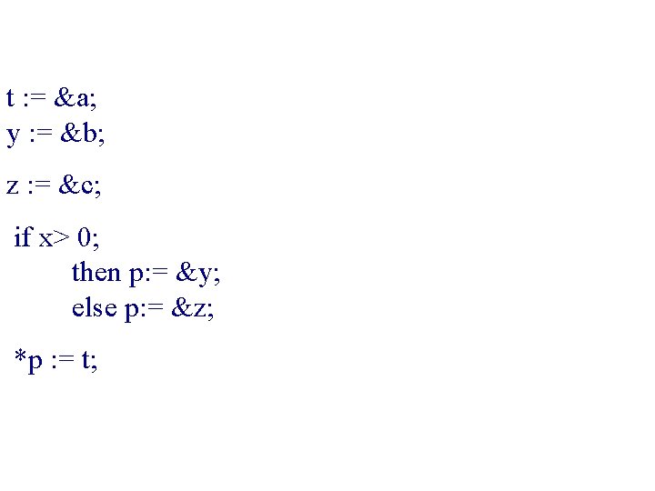
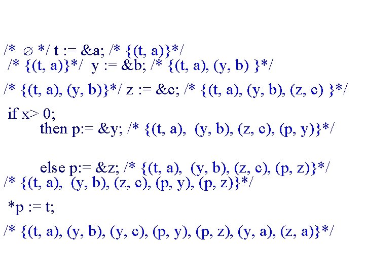
The PWhile Programming Language Abstract Syntax a : = x | *x | &x | n | a 1 opa a 2 b : = true | false | not b | b 1 opb b 2 | a 1 opr a 2 S : = x : = a | *x : = a | skip | S 1 ; S 2 | if b then S 1 else S 2 | while b do S
![Concrete Semantics 1 for PWhile State 1= [Loc Z] For every atomic statement S](http://slidetodoc.com/presentation_image_h/a6533b7be3a34d45f0a55be12528e9a1/image-37.jpg "Concrete Semantics 1 for PWhile State 1= [Loc Z] For every atomic statement S")
Concrete Semantics 1 for PWhile State 1= [Loc Z] For every atomic statement S S : States 1 x : = a ( )= [loc(x) A a ] x : = &y ( ) x : = *y ( ) x : = y ( )

Points-To Analysis u Lattice Lpt = u Galois connection
 x")
Abstract Semantics for PWhile • For every atomic statement S S #: P(Var*) x : = &y # x : = *y # x : = y # *x : = y #

Flow insensitive points-to-analysis Steengard 1996 u Ignore control flow u One set of points-to per program u Can be represented as a directed graph u Conservative approximation – Accumulate pointers u Can be computed in almost linear time

 = DF on all programs u")
Precision u We cannot usually have – (CS) = DF on all programs u But can we say something about precision in all programs? u Precision criteria – Join over all paths – Induced analysis

Summary u Abstract interpretation Connects Abstract and Concrete Semantics u Galois Connection u Local Correctness u Global Correctness
- Slides: 45