Iterative Computer Algorithms and their applications in engineering

Iterative Computer Algorithms: and their applications in engineering Sadiq M. Sait, Ph. D sadiq@kfupm. edu. sa Department of Computer Engineering King Fahd University of Petroleum and Minerals Dhahran, Saudi Arabia Special Talk for Motorola CAD Group, 1 Austin

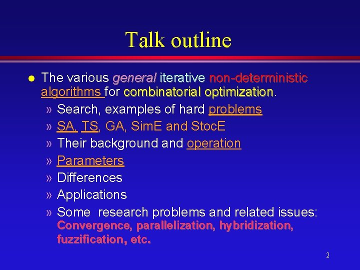
Talk outline l The various general iterative non-deterministic algorithms for combinatorial optimization » Search, examples of hard problems » SA, TS, GA, Sim. E and Stoc. E » Their background and operation » Parameters » Differences » Applications » Some research problems and related issues: Convergence, parallelization, hybridization, fuzzification, etc. 2

Talk outline Based on the text book by Sadiq M. Sait and Habib Youssef entitled: Iterative Computer Algorithms: and their applications in engineering to be published by IEEE Computer Society Press, 1999. 3

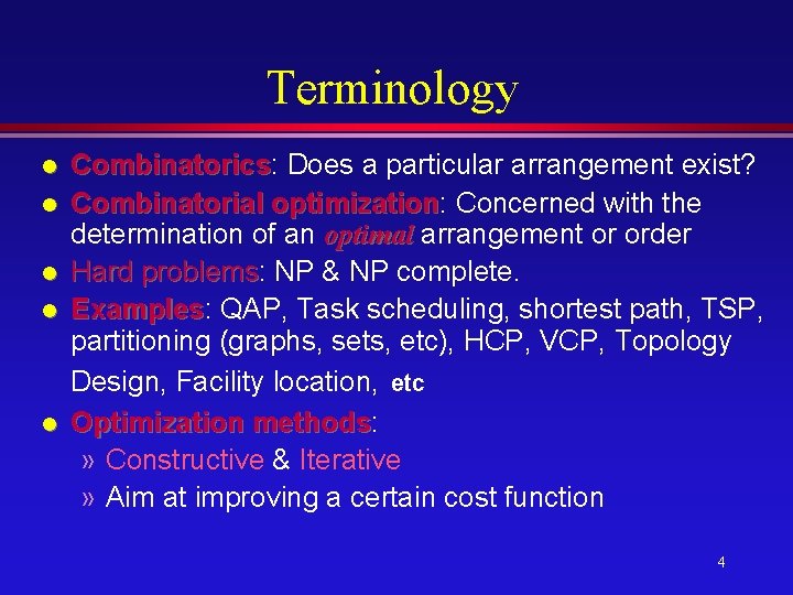
Terminology l l l Combinatorics: Combinatorics Does a particular arrangement exist? Combinatorial optimization: optimization Concerned with the determination of an optimal arrangement or order Hard problems: problems NP & NP complete. Examples: Examples QAP, Task scheduling, shortest path, TSP, partitioning (graphs, sets, etc), HCP, VCP, Topology Design, Facility location, etc Optimization methods: methods » Constructive & Iterative » Aim at improving a certain cost function 4

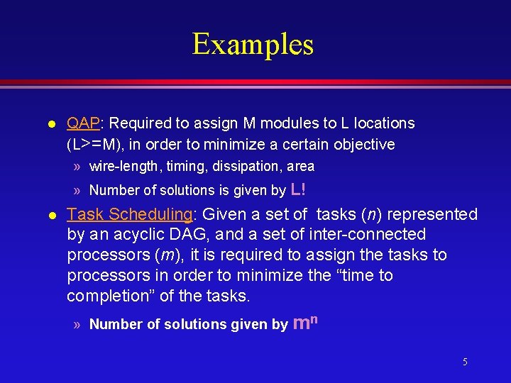
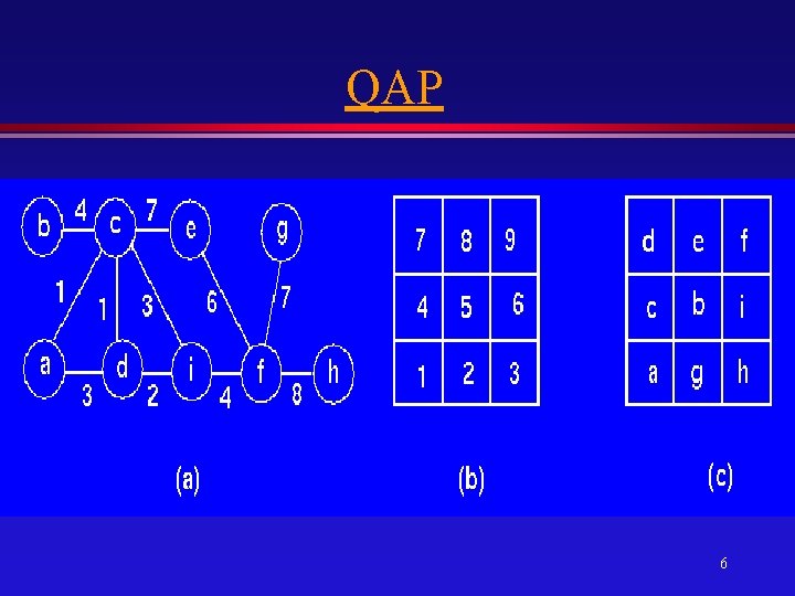
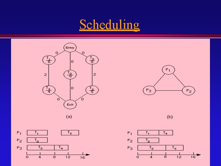
Examples l QAP: Required to assign M modules to L locations (L>=M), in order to minimize a certain objective » wire-length, timing, dissipation, area » Number of solutions is given by L! l Task Scheduling: Given a set of tasks (n) represented by an acyclic DAG, and a set of inter-connected processors (m), it is required to assign the tasks to processors in order to minimize the “time to completion” of the tasks. » Number of solutions given by mn 5

QAP 6

Scheduling 7

Purpose l To motivate application of iterative search heuristics to hard practical engineering problems. l To understand some of the underlying principles, parameters, and operators, of these modern heuristics. 8

Terminology l l l Search space Move (perturb function) Neighborhood Non-deterministic algorithms Optimal/Minimal solution 9

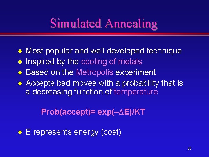
Simulated Annealing l l Most popular and well developed technique Inspired by the cooling of metals Based on the Metropolis experiment Accepts bad moves with a probability that is a decreasing function of temperature Prob(accept)= exp(– E)/KT l E represents energy (cost) 10

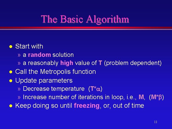
The Basic Algorithm l Start with » a random solution » a reasonably high value of T (problem dependent) l l Call the Metropolis function Update parameters » Decrease temperature (T* ) » Increase number of iterations in loop, i. e. , M, (M* ) l Keep doing so until freezing, or, out of time 11

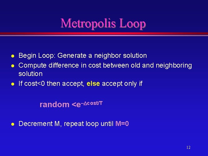
Metropolis Loop l l l Begin Loop: Generate a neighbor solution Compute difference in cost between old and neighboring solution If cost<0 then accept, else accept only if random <e– cost/T l Decrement M, repeat loop until M=0 12

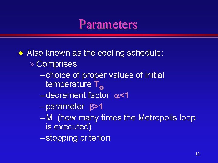
Parameters l Also known as the cooling schedule: » Comprises – choice of proper values of initial temperature To – decrement factor <1 – parameter >1 – M (how many times the Metropolis loop is executed) – stopping criterion 13

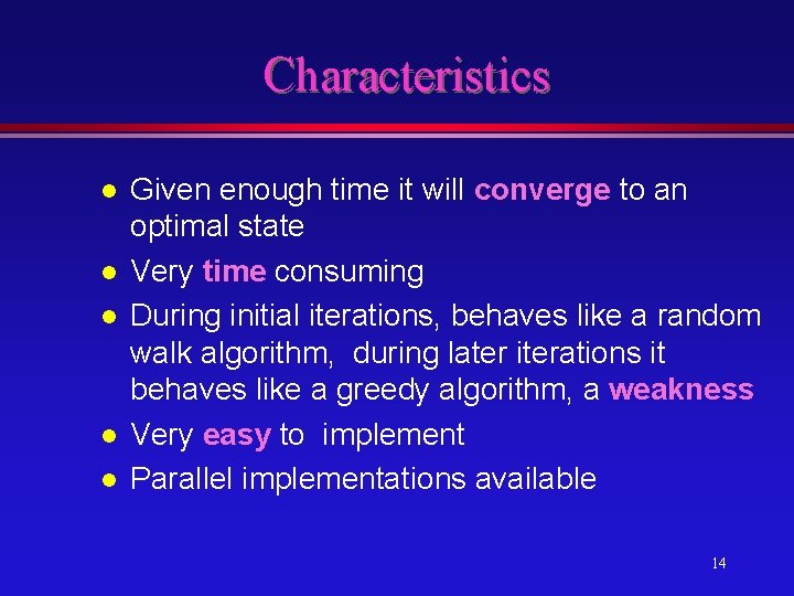
Characteristics l l l Given enough time it will converge to an optimal state Very time consuming During initial iterations, behaves like a random walk algorithm, during later iterations it behaves like a greedy algorithm, a weakness Very easy to implement Parallel implementations available 14

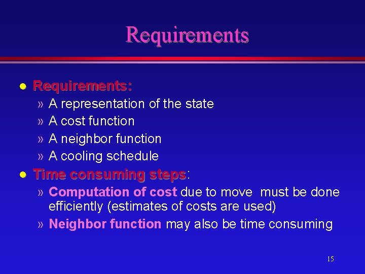
Requirements l Requirements: » A representation of the state » A cost function » A neighbor function » A cooling schedule l Time consuming steps: steps » Computation of cost due to move must be done efficiently (estimates of costs are used) » Neighbor function may also be time consuming 15

Applications l Has been successfully applied to a large number of combinatorial optimization problems in » science » engineering » medicine » business » etc 16

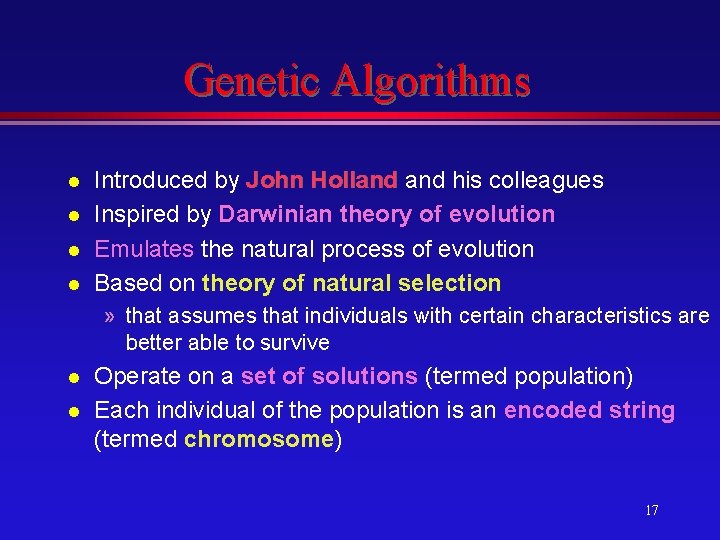
Genetic Algorithms l l Introduced by John Holland his colleagues Inspired by Darwinian theory of evolution Emulates the natural process of evolution Based on theory of natural selection » that assumes that individuals with certain characteristics are better able to survive l l Operate on a set of solutions (termed population) Each individual of the population is an encoded string (termed chromosome) 17

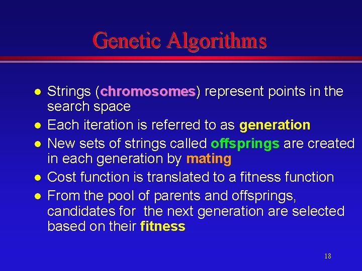
Genetic Algorithms l l l Strings (chromosomes) chromosomes represent points in the search space Each iteration is referred to as generation New sets of strings called offsprings are created in each generation by mating Cost function is translated to a fitness function From the pool of parents and offsprings, candidates for the next generation are selected based on their fitness 18

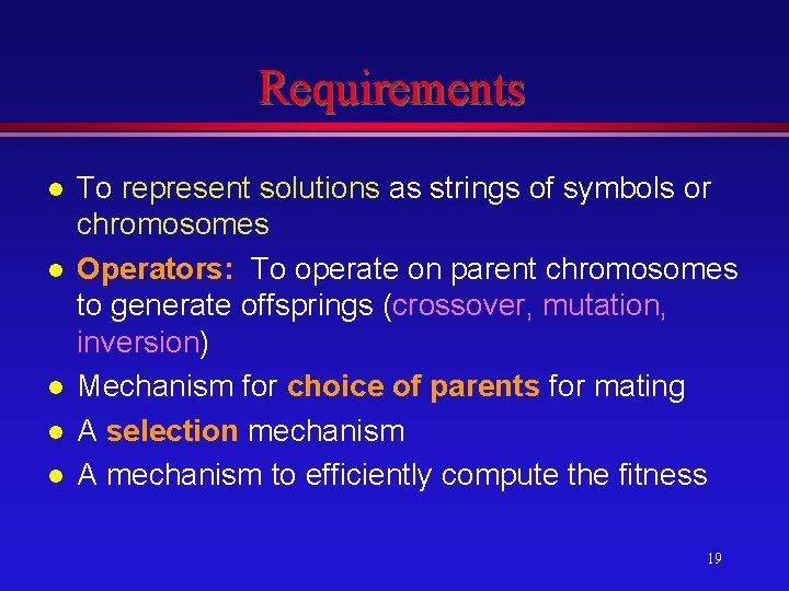
Requirements l l l To represent solutions as strings of symbols or chromosomes Operators: To operate on parent chromosomes to generate offsprings (crossover, mutation, inversion) Mechanism for choice of parents for mating A selection mechanism A mechanism to efficiently compute the fitness 19

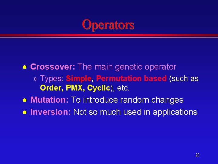
Operators l Crossover: The main genetic operator » Types: Simple, Permutation based (such as Order, PMX, Cyclic), etc. l l Mutation: To introduce random changes Inversion: Not so much used in applications 20

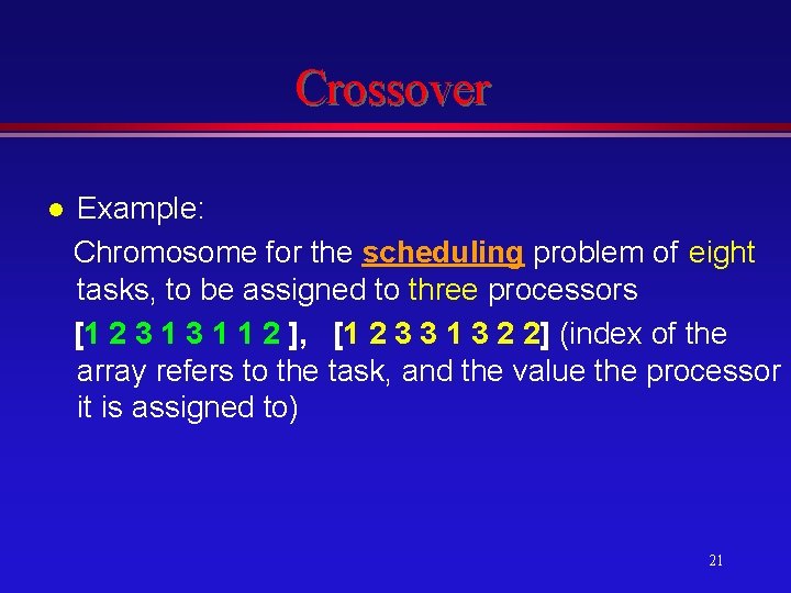
Crossover l Example: Chromosome for the scheduling problem of eight tasks, to be assigned to three processors [1 2 3 1 1 2 ], [1 2 3 3 1 3 2 2] (index of the array refers to the task, and the value the processor it is assigned to) 21

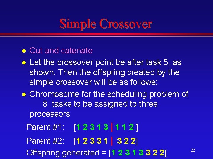
Simple Crossover l l l Cut and catenate Let the crossover point be after task 5, as shown. Then the offspring created by the simple crossover will be as follows: Chromosome for the scheduling problem of 8 tasks to be assigned to three processors Parent #1: [1 2 3 1 3 1 1 2 ] Parent #2: [1 2 3 3 1 3 2 2] Offspring generated = [1 2 3 1 3 3 2 2] 22

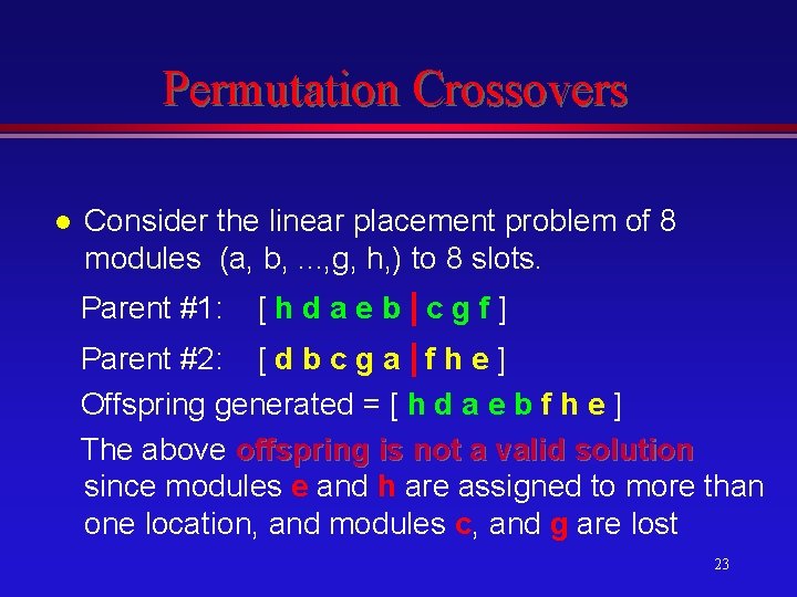
Permutation Crossovers l Consider the linear placement problem of 8 modules (a, b, . . . , g, h, ) to 8 slots. Parent #1: [hdaeb cgf] Parent #2: [ d b c g a f h e ] Offspring generated = [ h d a e b f h e ] The above offspring is not a valid solution since modules e and h are assigned to more than one location, and modules c, and g are lost 23

Order Crossovers Parent #1: [hdaeb cgf ] Parent #2: [dbfca ghe] Offspring generated = [ h d a e b f c g ] The above offspring represents a valid solution 24

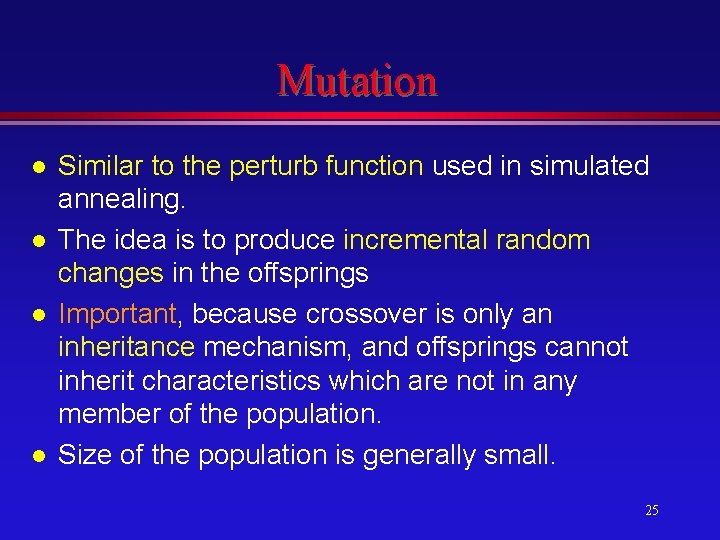
Mutation l l Similar to the perturb function used in simulated annealing. The idea is to produce incremental random changes in the offsprings Important, because crossover is only an inheritance mechanism, and offsprings cannot inherit characteristics which are not in any member of the population. Size of the population is generally small. 25

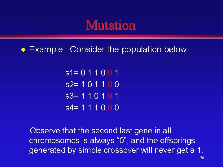
Mutation l Example: Consider the population below s 1= 0 1 1 0 0 1 s 2= 1 0 1 1 0 0 s 3= 1 1 0 1 s 4= 1 1 1 0 0 0 Observe that the second last gene in all chromosomes is always “ 0”, and the offsprings generated by simple crossover will never get a 1. 26

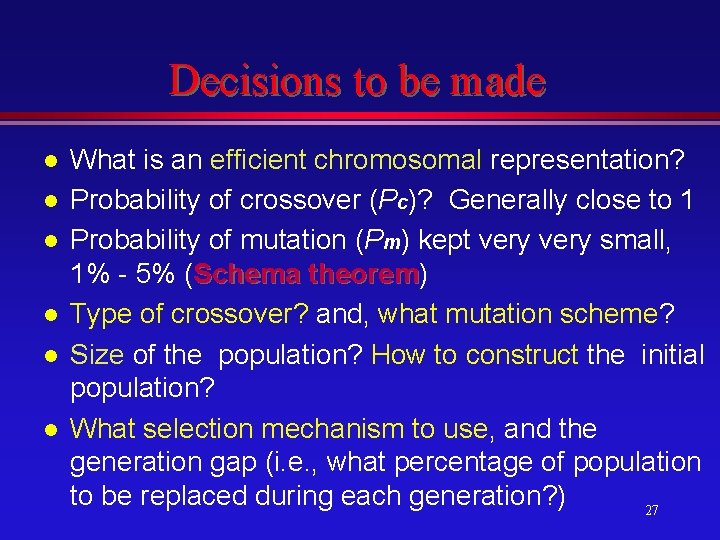
Decisions to be made l l l What is an efficient chromosomal representation? Probability of crossover (Pc)? Generally close to 1 Probability of mutation (Pm) kept very small, 1% - 5% (Schema theorem) theorem Type of crossover? and, what mutation scheme? Size of the population? How to construct the initial population? What selection mechanism to use, and the generation gap (i. e. , what percentage of population to be replaced during each generation? ) 27

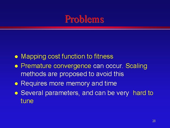
Problems l l Mapping cost function to fitness Premature convergence can occur. Scaling methods are proposed to avoid this Requires more memory and time Several parameters, and can be very hard to tune 28

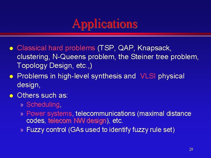
Applications l l l Classical hard problems (TSP, QAP, Knapsack, clustering, N-Queens problem, the Steiner tree problem, Topology Design, etc. , ) Problems in high-level synthesis and VLSI physical design, Others such as: » Scheduling, » Power systems, telecommunications (maximal distance codes, telecom NW design), design etc. » Fuzzy control (GAs used to identify fuzzy rule set) 29

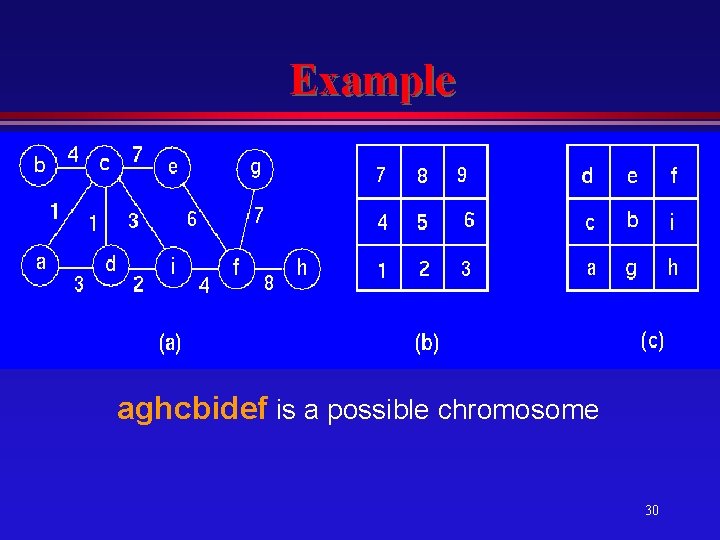
Example aghcbidef is a possible chromosome 30

Some Variations l l l l 2 -D chromosomes Gray versus Binary encoding Multi-objective optimization with GAs Constant versus dynamically decreasing population Niches, crowding and speciation Scaling etc 31

Tabu Search l l Introduced by Fred Glover Generalization of Local Search At each step, the local neighborhood of the current solution is explored and the best solution is selected as the next solution This best neighbor solution is accepted even if it is worse than the current solution (hill climbing) 32

Central Idea l l Exploitation of memory structures Short term memory » Tabu list » Aspiration criterion Intermediate memory for intensification Long term memory for diversification 33

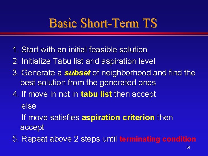
Basic Short-Term TS 1. Start with an initial feasible solution 2. Initialize Tabu list and aspiration level 3. Generate a subset of neighborhood and find the best solution from the generated ones 4. If move in not in tabu list then accept else If move satisfies aspiration criterion then accept 5. Repeat above 2 steps until terminating condition 34

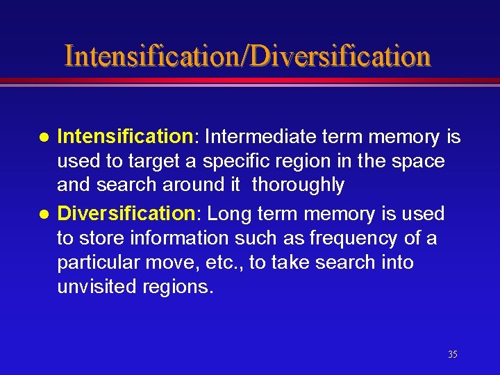
Intensification/Diversification l l Intensification: Intermediate term memory is used to target a specific region in the space and search around it thoroughly Diversification: Long term memory is used to store information such as frequency of a particular move, etc. , to take search into unvisited regions. 35

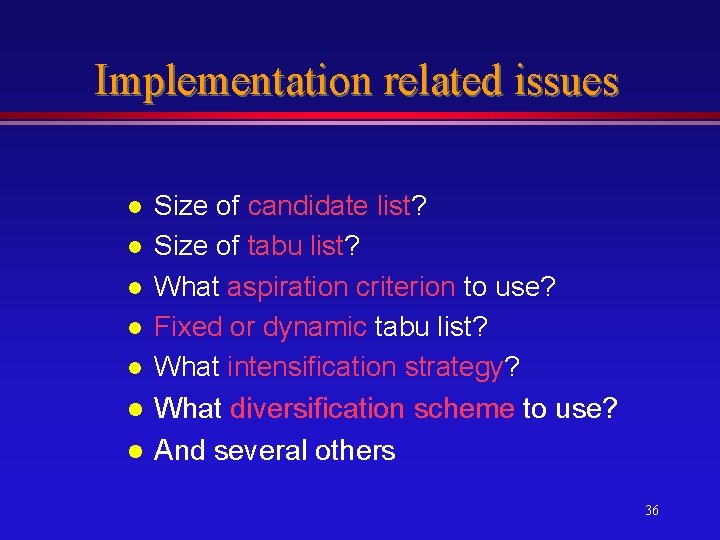
Implementation related issues l l l l Size of candidate list? Size of tabu list? What aspiration criterion to use? Fixed or dynamic tabu list? What intensification strategy? What diversification scheme to use? And several others 36

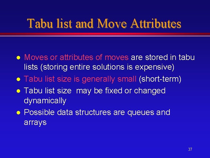
Tabu list and Move Attributes l l Moves or attributes of moves are stored in tabu lists (storing entire solutions is expensive) Tabu list size is generally small (short-term) Tabu list size may be fixed or changed dynamically Possible data structures are queues and arrays 37

Related Issues l l l l Design of evaluator functions Candidate list strategies Target analysis Strategic oscillation Path relinking Parallel implementation Convergence aspects Applications (again several) 38

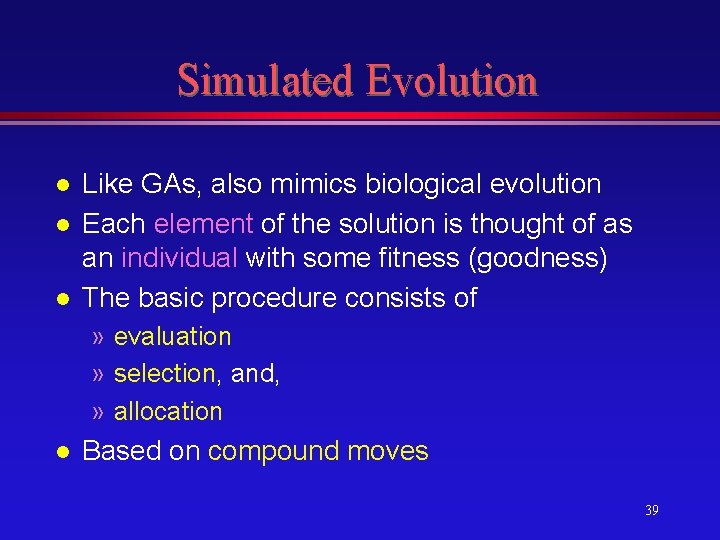
Simulated Evolution l l l Like GAs, also mimics biological evolution Each element of the solution is thought of as an individual with some fitness (goodness) The basic procedure consists of » evaluation » selection, and, » allocation l Based on compound moves 39

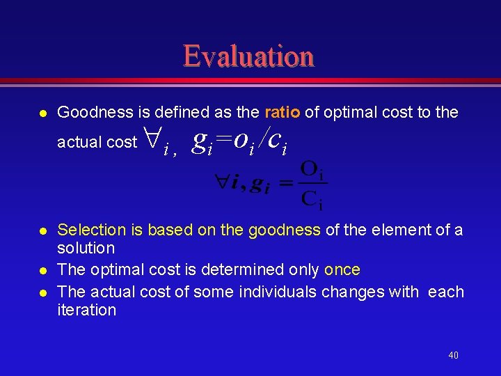
Evaluation l Goodness is defined as the ratio of optimal cost to the actual cost l l l i , gi=oi /ci Selection is based on the goodness of the element of a solution The optimal cost is determined only once The actual cost of some individuals changes with each iteration 40

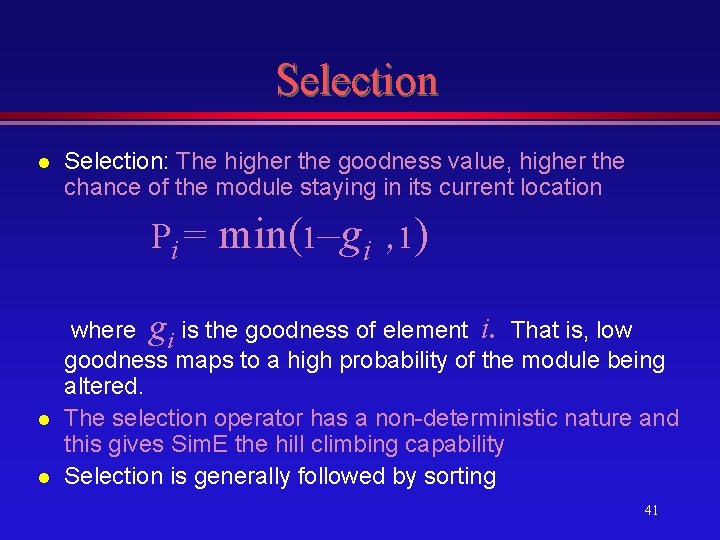
Selection l Selection: The higher the goodness value, higher the chance of the module staying in its current location Pi = min(1–gi , 1). l l where gi is the goodness of element i That is, low goodness maps to a high probability of the module being altered. The selection operator has a non-deterministic nature and this gives Sim. E the hill climbing capability Selection is generally followed by sorting 41

Allocation l l l This is a complex form of genetic mutation (compound move) This operator takes two sets (selection S and remaining set R) and generates a new population Has the most impact on the rate of convergence 42

Comparison of Sim. E and SA l l l In SA a perturbation is a single move For SA, the elements to be moved are selected at random SA is guided by a parameter called temperature, while for Sim. E the search is guided by the individual fitness of the solution components 43

Comparison of Sim. E and GA l l l Sim. E works on a single solution called population while in GA, the set of solutions comprises the population GA relies on genetic reproduction (using crossover, mutation, etc). In Sim. E, an individual is evaluated by estimating the fitness of each of its genes. (Genes with lower fitness have a higher probability of getting altered) 44

Other facts l l Fairly simple, yet very powerful Has been applied to several hard problems (such as VLSI standard cell placement, high level synthesis, etc) Parallel implementations have been proposed (for MISD and MIMD) Convergence analysis presented by designers of the heuristic and others 45

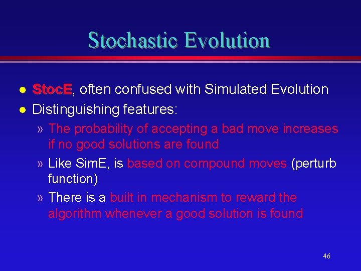
Stochastic Evolution l l Stoc. E, Stoc. E often confused with Simulated Evolution Distinguishing features: » The probability of accepting a bad move increases if no good solutions are found » Like Sim. E, is based on compound moves (perturb function) » There is a built in mechanism to reward the algorithm whenever a good solution is found 46

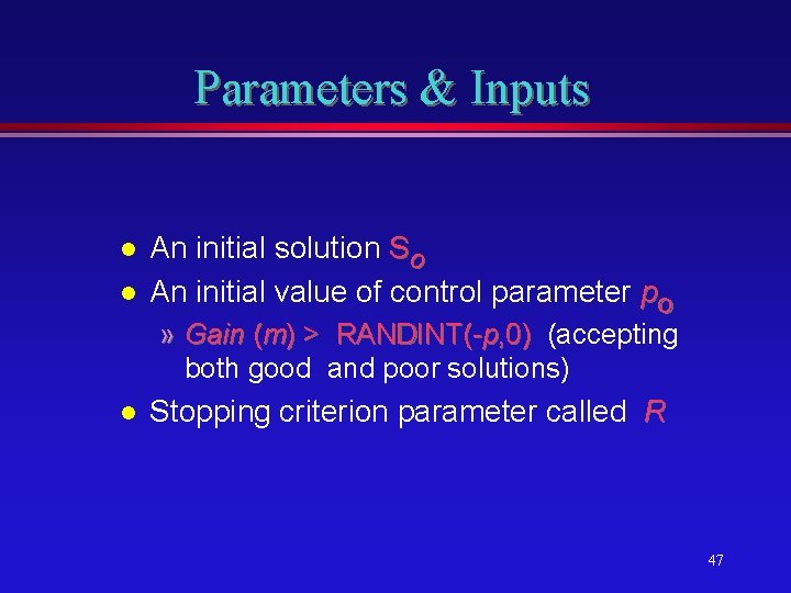
Parameters & Inputs l l An initial solution So An initial value of control parameter po » Gain (m) > RANDINT(-p, 0) (accepting both good and poor solutions) l Stopping criterion parameter called R 47

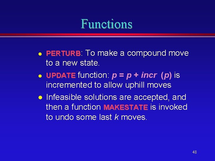
Functions l l l PERTURB: To make a compound move to a new state. UPDATE function: p = p + incr (p) is incremented to allow uphill moves Infeasible solutions are accepted, and then a function MAKESTATE is invoked to undo some last k moves. 48

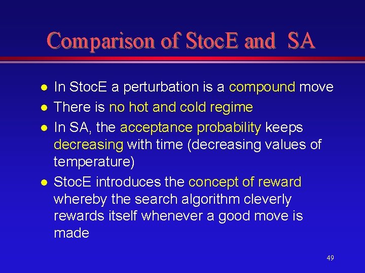
Comparison of Stoc. E and SA l l In Stoc. E a perturbation is a compound move There is no hot and cold regime In SA, the acceptance probability keeps decreasing with time (decreasing values of temperature) Stoc. E introduces the concept of reward whereby the search algorithm cleverly rewards itself whenever a good move is made 49

Common features of All heuristics l l l l All are general iterative heuristics, can be applied to any combinatorial optimization problem All are conceptually simple and elegant All are based on moves and neighborhood All are blind All occasionally accept inferior solutions (i. e, have hill-climbing capability) All are non-deterministic (except TS which is only to some extent) “All” (under certain conditions) asymptotically converge to an optimal solution (TS and Stoc. E)50

Some Research Areas l l l Applications to various hard problems of current technology? Hybridization? » How to enhance strengths and compensate for weaknesses of two or more heuristics » Examples: SA/TS, GA/SA, TS/Sim. E, etc Fuzzy logic for multi-objective optimization and other operations. Parallel implementations Convergence aspects 51

52