ISE 203 OR I Chapter 3 Introduction to

ISE 203 OR I Chapter 3 Introduction to Linear Programming Asst. Prof. Dr. Nergiz Kasımbeyli 1

Linear Programming 2

An Example 3

The Data Gathered 4

Definition of the Problem Determine what the production rates should be for the two products in order to maximize their total profit, subject to the restrictions imposed by the limited production capacities available in the three plants. 5

Data for the Problem 6

Formulation as a Linear Programming Model • Decision Variables: x 1 = number of batches of product 1 produced per week x 2 = number of batches of product 2 produced per week • Objective Function: Maximize Z = total profit per week (in thousands) from producing these two products 7

LP Formulation 8

Graphical Solution Since the LP has only two decision variables (two dimensions), the problem can be solved graphically. Let’s identify the values of x 1 and x 2 that are permitted by the constraints. Constraint 1: x 1 ≤ 4 9

The Feasible Region Constraint 1: x 1 ≤ 4 Constraint 2: 2 x 2 ≤ 12 Constraint 3: 3 x 1 + 2 x 2 = 18 Constraints 4 and 5: x 1 ≥ 0 , x 2 ≥ 0 10

Maximizing the value of Z Slope of the objective function line = -3/5 11

Optimal Solution 12

• The Optimal solution is x 1 = 2, x 2 = 6 with Z = 36. • This solution indicates that the Wyndor Glass Co. should produce products 1 and 2 at the rate of 2 batches per week and 6 batches per week, respectively, with a resulting total profit of $36, 000 per week. 13

14

Standard form of the model 15

16

17

Terminology for Solutions of the Model 18

No feasible solution

Multiple optimal solutions 20

Unbounded objective: No optimal solution 21

CPF: Corner-point feasible solution 5 CPF solutions are shown in the figure. Other equivalent terms: • Extreme points • Vertices 22

IMPORTANT: Relationship between CPF solutions and optimal solutions: • The best CPF solution must be an optimal solution. àIf a problem has exactly one optimal solution, it must be a CPF solution. àIf a problem has multiple optimal solutions, at least two must be CPF solutions. 23

24

Proportionality assumption 25

Proportionality assumption-Case 1 26

Proportionality assumption-Case 2 (increasing marginal return) 27

Decreasing marginal return-Case 3 28

29

Z = 3 x 1 + 5 x 2 + x 1 x 2 Z = 3 x 1 + 5 x 2 - x 1 x 2

3 x 1 + 2 x 2 ≤ 18 3 x 1 + 2 x 2 + 0. 5 x 1 x 2 ≤ 18 3 x 1 + 2 x 2 + 0. 1 x 12 x 2 ≤ 18

Example: Giapetto’s Woodcarving • Giapetto’s, Inc. , manufactures wooden soldiers and trains. – Each soldier built: • • Sell for $27 and uses $10 worth of raw materials. Increase Giapetto’s variable labor/overhead costs by $14. Requires 2 hours of finishing labor. Requires 1 hour of carpentry labor. – Each train built: • • Sell for $21 and used $9 worth of raw materials. Increases Giapetto’s variable labor/overhead costs by $10. Requires 1 hour of finishing labor. Requires 1 hour of carpentry labor.

• Each week Giapetto can obtain: – All needed raw material. – Only 100 finishing hours. – Only 80 carpentry hours. • Demand for the trains is unlimited. • At most 40 soldiers are bought each week. • Giapetto wants to maximize weekly profit (revenues – costs). • Formulate a mathematical model of Giapetto’s situation that can be used maximize weekly profit.

Solution • The Giapetto solution model incorporates the characteristics shared by all linear programming problems. – Decision variables should completely describe the decisions to be made. • x 1 = number of soldiers produced each week • x 2 = number of trains produced each week – The decision maker wants to maximize (usually revenue or profit) or minimize (usually costs) some function of the decision variables. This function to maximized or minimized is called the objective function.

Solution continued • Giapetto’s weekly profit can be expressed in terms of the decision variables x 1 and x 2: Weekly profit = weekly revenue – weekly raw material costs – the weekly variable costs = 3 x 1 + 2 x 2 • Thus, Giapetto’s objective is to chose x 1 and x 2 to maximize weekly profit. The variable z denotes the objective function value of any LP. • Giapetto’s objective function is Maximize z = 3 x 1 + 2 x 2 • The coefficient of an objective function variable is called an objective function coefficient.

Solution continued • As x 1 and x 2 increase, Giapetto’s objective function grows larger. • For Giapetto, the values of x 1 and x 2 are limited by the following three restrictions (constraints): – Each week, no more than 100 hours of finishing time may be used. (2 x 1 + x 2 ≤ 100) – Each week, no more than 80 hours of carpentry time may be used. (x 1 + x 2 ≤ 80) – Because of limited demand, at most 40 soldiers should be produced. (x 1 ≤ 40)

• The coefficients of the decision variables in the constraints are called the technological coefficients. The number on the right-hand side of each constraint is called the constraint’s right-hand side (or rhs). • To complete the formulation of a linear programming problem, the following question must be answered for each decision variable. – Can the decision variable only assume nonnegative values, or is the decision variable allowed to assume both positive and negative values? • If the decision variable can assume only nonnegative values, the sign restriction xi ≥ 0 is added. • If the variable can assume both positive and negative values, the decision variable xi is unrestricted in sign (often abbreviated urs).

Solution continued • For the Giapetto problem model, combining the sign restrictions x 1≥ 0 and x 2≥ 0 with the objective function and constraints yields the following optimization model: Max z = 3 x 1 + 2 x 2 (objective function) Subject to (s. t. ) 2 x 1 + x 2 ≤ 100 (finishing constraint) x 1 + x 2 ≤ 80 (carpentry constraint) x 1 ≤ 40 (constraint on demand for soldiers) x 1 ≥ 0 (sign restriction) x 2

• The set of points satisfying the Giapetto LP is bounded by the five sided polygon DGFEH. Any point on or in the interior of this polygon (the shade area) is in the feasible region. Optimal solution x 1 =20, x 2 =60

• Having identified the feasible region for the Giapetto LP, a search can begin for the optimal solution which will be the point in the feasible region with the largest z-value. • To find the optimal solution, graph a line on which the points have the same z-value. In a max problem, such a line is called an isoprofit line while in a min problem, this is called the isocost line. The figure shows the isoprofit lines for z = 60, z = 100, and z = 180.

• A constraint is binding if the left-hand right-hand side of the constraint are equal when the optimal values of the decision variables are substituted into the constraint. – In the Giapetto LP, the finishing and carpentry constraints are binding. • A constraint is nonbinding if the left-hand side and the right-hand side of the constraint are unequal when the optimal values of the decision variables are substituted into the constraint. – In the Giapetto LP, the demand constraint for wooden soldiers is nonbinding since at the optimal solution (x 1 = 20), x 1 < 40.

• A set of points S is a convex set if the line segment jointing any two pairs of points in S is wholly contained in S. • For any convex set S, a point P in S is an extreme point if each line segment that lies completely in S and contains the point P has P as an endpoint of the line segment. – The feasible region for the Giapetto LP will be a convex set.

Example: Dorian Auto • Dorian Auto manufactures luxury cars and trucks. • The company believes that its most likely customers are high-income women and men. • To reach these groups, Dorian Auto has embarked on an ambitious TV advertising campaign and will purchase 1 -minute commercial spots on two type of programs: comedy shows and football games.

• Each comedy commercial is seen by 7 million high income women and 2 million high-income men and costs $50, 000. • Each football game is seen by 2 million high-income women and 12 million high-income men and costs $100, 000. • Dorian Auto would like for commercials to be seen by at least 28 million high-income women and 24 million high-income men. • Use LP to determine how Dorian Auto can meet its advertising requirements at minimum cost.

Dorian: Solution • Dorian must decide how many comedy and football ads should be purchased, so the decision variables are – x 1 = number of 1 -minute comedy ads – x 2 = number of 1 -minute football ads • Dorian wants to minimize total advertising cost. • Dorian’s objective functions is min z = 50 x 1 + 100 x 2 • Dorian faces the following the constraints – Commercials must reach at least 28 million high-income women. (7 x 1 + 2 x 2 ≥ 28) – Commercials must reach at least 24 million high-income men. (2 x 1 + 12 x 2 ≥ 24) – The sign restrictions are necessary, so x 1, x 2 ≥ 0.

Solution continued To solve this LP graphically begin by graphing the feasible region.

Solution continued • Like the Giapetto LP, The Dorian LP has a convex feasible region. • The feasible region for the Dorian problem, however, contains points for which the value of at least one variable can assume arbitrarily large values. • Such a feasible region is called an unbounded feasible region.

Solution continued • Since Dorian wants to minimize total advertising costs, the optimal solution to the problem is the point in the feasible region with the smallest z value. • An isocost line with the smallest z value passes through point E and is the optimal solution at x 1 = 3. 4 and x 2 = 1. 4. • Both the high-income women and high-income men constraints are satisfied, both constraints are binding.

• Does the Dorian problem meet the four assumptions of linear programming? • The Proportionality Assumption is violated because at a certain point advertising will yield diminishing returns. • Even though the Additivity Assumption was used in writing: (Total viewers) = (Comedy viewer ads) + (Football ad viewers) many of the same people might view both ads, double-counting of such people would occur thereby violating the assumption. • The Divisibility Assumption is violated if only 1 -minute commercials are available. Dorian is unable to purchase 3. 6 comedy and 1. 4 football commercials. • The Certainty assumption is also violated because there is no way to know with certainty how many viewers are added by each type of commercial.

Example: Diet Problem • My diet requires that all the food I get come from one of the four “basic food groups”. • At present, the following four foods are available for consumption: brownies, chocolate ice cream, cola and pineapple cheesecake. • Each brownie costs 50¢, each scoop of ice cream costs 20 ¢, each bottle of cola costs 30 ¢, and each piece of pineapple cheesecake costs 80 ¢. • Each day, I must ingest at least 500 calories, 6 oz of chocolate, 10 oz of sugar, and 8 oz of fat. • The nutritional content per unit of each food is given. • Formulate a linear programming model that can be used to satisfy my daily nutritional requirements at minimum cost.

Nutritional Values for Diet Calories Chocolate (ounces) Sugar (ounces) Fat (ounces) Brownie 400 3 2 2 Chocolate Ice Cream (1 scoop) 200 2 2 4 Cola (1 bottle) 250 0 4 1 Pineapple Cheesecake (1 piece) 500 0 4 5

Solution • As always, begin by determining the decisions that must be made by the decision maker: how much of each type of food should be eaten daily. • Thus we define the decision variables: – – x 1 = number of brownies eaten daily x 2 = number of scoops of chocolate ice cream eaten daily x 3 = bottles of cola drunk daily x 4 = pieces of pineapple cheesecake eaten daily

Solution continued • My objective is to minimize the cost of my diet. • The total cost of any diet may be determined from the following relation: (total cost of diet) = (cost of brownies) + (cost of ice cream) +(cost of cola) + (cost of cheesecake). • The decision variables must satisfy the following four constraints: – – Daily calorie intake must be at least 500 calories. Daily chocolate intake must be at least 6 oz. Daily sugar intake must be at least 10 oz. Daily fat intake must be at least 8 oz.

Solution continued • Express each constraint in terms of the decision variables. • The optimal solution to this LP is found by combining the objective functions, constraints, and the sign restrictions. (Can you find the solution graphically? ) • The chocolate and sugar constraints are binding, but the calories and fat constraints are nonbinding. • A version of the diet problem with a more realistic list of foods and nutritional requirements was one of the first LPs to be solved by computer.

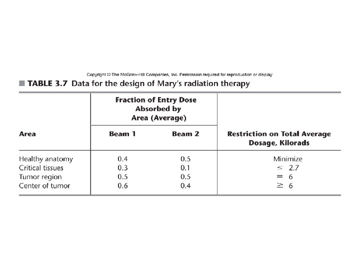
Additional Examples Design of Radiation Therapy

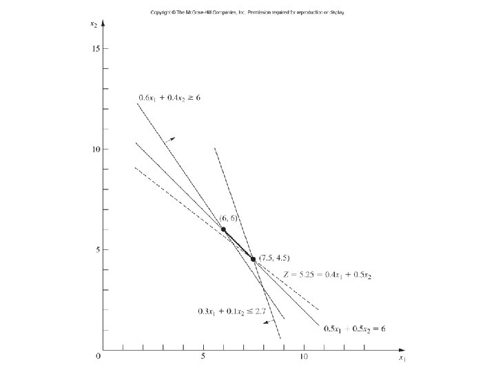
LP Formulation Decision Variables: x 1: dose (in kilorads) at the entry point for beam 1 x 2: dose (in kilorads) at the entry point for beam 1 Minimize Z=0. 4 x 1 + 0. 5 x 2 s. t. 0. 3 x 1 + 0. 1 x 2 ≤ 2. 7 0. 5 x 1 + 0. 5 x 2 = 6 0. 6 x 1 + 0. 4 x 2 ≥ 6 x 1 ≥ 0, x 2 ≥ 0 57

Personnel Scheduling 59

The problem is to determine how many agents should be assigned to the respective shifts each day to minimize the total personnel cost for agents. 60

LP Formulation: Redundant constraints 61