Investments Analysis and Behavior Chapter 5 Asset Pricing

Learning Objectives n n n Know theory and application of the CAPM. Learn multifactor pricing models. Realize the limitations of asset pricing models. Assess the performance of a portfolio. Compute alpha, Sharpe, and Treynor measures 5 -2

Capital Asset Pricing Model (CAPM) n Elegant theory of the relationship between risk and return ¨ Used for asset pricing ¨ Risk evaluation ¨ Assessing portfolio performance ¨ William Sharpe won the Nobel Prize in Economics in 1990 n Empirical record is poor 5 -3

CAPM Basic Assumptions n n n n Investors hold efficient portfolios—higher expected returns involve higher risk. Unlimited borrowing and lending is possible at the risk-free rate. Investors have homogenous expectations. There is a one-period time horizon. Investments are infinitely divisible. No taxes or transaction costs exist. Inflation is fully anticipated. Capital markets are in equilibrium. Examine CAPM as an extension to portfolio theory: 5 -4

5 -5

5 -6

5 -7

The Equation of the CML is: n Y = b + m. X This leads to the Security Market Line (SML) 5 -8

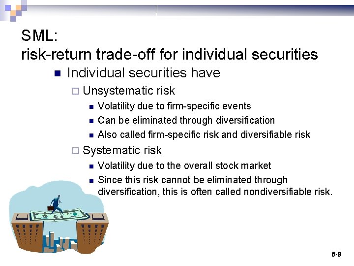
SML: risk-return trade-off for individual securities n Individual securities have ¨ Unsystematic n n n Volatility due to firm-specific events Can be eliminated through diversification Also called firm-specific risk and diversifiable risk ¨ Systematic n n risk Volatility due to the overall stock market Since this risk cannot be eliminated through diversification, this is often called nondiversifiable risk. 5 -9

5 -10

The equation for the SML leads to the CAPM β is a measure of relative risk β = 1 for the overall market. n β = 2 for a security with twice the systematic risk of the overall market, n β = 0. 5 for a security with one-half the systematic risk of the market. 5 -11 n

5 -12

Using CAPM n Expected Return ¨ If the market is expected to increase 10% and the risk free rate is 5%, what is the expected return of assets with beta=1. 5, 0. 75, and -0. 5? Beta = 1. 5; E(R) = 5% + 1. 5 (10% - 5%) = 12. 5% n Beta = 0. 75; E(R) = 5% + 0. 75 (10% - 5%) = 8. 75% n Beta = -0. 5; E(R) = 5% + -0. 5 (10% - 5%) = 2. 5% n n Finding Undervalued Stocks…(the SML) 5 -13

5 -14

CAPM and Portfolios n How does adding a stock to an existing portfolio change the risk of the portfolio? ¨ Standard Deviation as risk n Correlation of new stock to every other stock ¨ Beta n Simple weighted average: n n Existing portfolio has a beta of 1. 1 New stock has a beta of 1. 5. The new portfolio would consist of 90% of the old portfolio and 10% of the new stock New portfolio’s beta would be 1. 14 (=0. 9× 1. 1 + 0. 1× 1. 5) 5 -15

Estimating Beta n Need ¨ Risk free rate data ¨ Market portfolio data n S&P 500, DJIA, NASDAQ, etc. ¨ Stock n Interval ¨ n return data Daily, monthly, annual, etc. Length ¨ One year, five years, ten years, etc. 5 -16

Market Index variations Constant 0. 001 Std Err of Y Est 0. 005 R Squared 18. 67% R Squared 9. 94% No. of Observations 52 Degrees of Freedom 50 Beta estimate Std Err of Coef. t-statistic 1. 19 0. 351 3. 39 Beta estimate 0. 549 Std Err of Coef. 0. 233 t-statistic 2. 356 5 -17

Interval variations Constant 0. 0001 Constant 0. 017 Std Err of Y Est 0. 0002 Std Err of Y Est 0. 054 R Squared 33. 09% R Squared 31. 79% No. of Observations 9090 No. of Observations 36 Degrees of Freedom 9088 Degrees of Freedom 34 Beta estimate 1. 039 Beta estimate 1. 258 Std Err of Coef. 0. 016 Std Err of Coef. 0. 316 t-statistic 67. 07 t-statistic 3. 98 5 -18

Problems using Beta n n Which market index? Which time intervals? Time length of data? Non-stationary Beta estimates of a company change over time. ¨ How useful is the beta you estimate now for thinking about the future? ¨ n Other factors seem to have a stronger empirical relationship between risk and return than beta Not allowed in CAPM theory ¨ Size and B/M ¨ 5 -19

Multifactor models n Arbitrage Pricing Theory (APT) ¨ Multiple n n risk factors, one of which may be beta What are these factors, F 1, F 2, etc. ? Unexpected inflation, risk yield spread, oil prices, … ¨ Example n n Specify an APT model with three factors; the CAPM beta (F 1), unexpected inflation (F 2), and the risk yield spread (F 3). A company being analyzed has risk factor sensitivities of b 1 = 1. 2, b 2 = -2. 2, and b 3 = 0. 1. The intercept, α, was 3. 5%. The risk premium on the market was 5%, unexpected inflation turned out to be +2%, and the yield spread is 4%, what risk premium should the company have earned? n 5 -20

Multifactor models n Fama-French Three Factor Model ¨ Beta, n n size, and B/M SMB, difference in returns of portfolio of small stocks and portfolio of large stocks HML, difference in return between low B/M portfolio and high B/M portfolio ¨ Kenneth French keeps a web site where you can obtain historical values of the Fama-French factors, mba. tuck. dartmouth. edu/pages/faculty/ken. french/data_library. html 5 -21

New Behavioral Approaches n The design of asset pricing models began using theories of rational investor behavior. ¨ Rational investors are generally thought to be risk averse, can fully exploit all available information, and do not suffer from psychological biases. ¨ The expected rate of return on investment for a given portfolio is solely a function of the economic risks faced. n Investors do not always act “rational ¨ Behavioral risk factors like the reluctance to realize losses, overconfidence, and momentum might be applied to asset pricing. 5 -22

Add a momentum factor… Those that follow behavioral finance might argue that the SMB factor is actually a Overreaction risk factor. n Also add a momentum factor: n The UMD (up minus down) momentum factor is the return on a portfolio of the best performing stocks minus the portfolio return for the worst stocks during the preceding twelve month period. 5 -23

Evaluating Portfolio Performance n How well did a portfolio manager do? ¨ Different portfolios take different levels of risk. n ¨ Some managers have constraints n n There they should earn different returns. Must invest in small cap stocks or a particular industry. Evaluation of a portfolio’s performance should therefore include: Risk-adjusted performance ¨ Comparisons with similarly constrained portfolios ¨ 5 -24

Benchmarks n Comparing the portfolio to similar portfolios ¨ Market benchmarks n S&P 500 Index: General market n S&P 100 Index: Large cap n S&P 400 Index: Mid cap n S&P 600 Index: Small cap ¨ n Russell 2000 Industry benchmarks ¨ Dow Jones US Technology Index, DJ US Financial, DJ US Health Care, … ¨ Managed Portfolio benchmarks n Average return of all mutual funds with the same constraints ¨ Small cap, value strategy, international, etc. 5 -25

Alpha n Given CAPM, a portfolio should earn the return of: E(RP) = RF + βP(RM - RF) ¨ So, if RF = 5%, βP = 1. 2, RM = 11% ¨ The return should be 12. 2% = 5%+ 1. 2×(11%-5%) ¨ If the portfolio earned 13%, then it did well. If it earned 11. 5%, it did poorly. Alpha is the difference between what it did earn and what is should have earned. αP = RP - RF - βP(RM - RF) n n Positive alphas are good! Alpha is an absolute measure of performance. ¨ What is the source of the n Selectivity: stock picking n Market timing non-zero alpha? 5 -26

Table 5. 2 Beta Estimation for Ten Large Mutual Funds Using the S&P 500 as a Market Index Alpha Mutual Fund Beta Ticker estimate t-statistic R sq. American Century Ultra TWCUX 0. 010 0. 12 0. 977 25. 69 92. 8% Fidelity Advisors Growth Opportunity FAGOX 0. 023 0. 48 1. 048 45. 86 97. 6% Fidelity Contrafund FCNTX 0. 153 1. 75 0. 717 17. 18 85. 3% Fidelity Magellan Fund FMAGX -0. 033 -1. 05 0. 995 66. 95 98. 9% Fidelity Puritan FPURX 0. 027 0. 45 0. 614 21. 15 89. 8% Investment Co. of America AIVSX 0. 050 0. 98 0. 759 30. 82 94. 9% Janus Fund JANSX 0. 038 0. 37 1. 084 22. 23 90. 7% Vanguard 500 Index VFINX -0. 003 -0. 19 1. 013 141. 42 99. 7% Vanguard Wellington VWELX 0. 039 0. 61 0. 601 19. 55 88. 2% Washington Mutual AWSHX -0. 025 -0. 45 0. 907 34. 09 95. 8% 0. 028 0. 307 0. 872 42. 494 93. 4% Averages Data source: http: //finance. yahoo. com (2003 data). 5 -27

Sharpe Ratio n Reward-to-variability measure ¨ Risk premium earned per unit of total risk: ¨ Higher Sharpe ratio is better. ¨ Use as a relative measure. n Portfolios are ranked by the Sharpe measure. 5 -28

Treynor Index n Reward-to-volatility measure ¨ Risk premium earned per unit of systematic risk: ¨ Higher Treynor Index is better. ¨ Use as a relative measure. 5 -29

Example n n n A pension fund’s average monthly return for the year was 0. 9% and the standard deviation was 0. 5%. The fund uses an aggressive strategy as indicated by its beta of 1. 7. If the market averaged 0. 7%, with a standard deviation of 0. 3%, how did the pension fund perform relative to the market? The monthly risk free rate was 0. 2%. Solution: n Compute and compare the Sharpe and Treynor measures of the fund and market. n For the pension fund: n For the market: n Both the Sharpe ratio and the Treynor Index are greater for the market than for the mutual fund. Therefore, the mutual fund under-performed the market. 5 -30

Summary n CAPM is an elegant model ¨ Used extensively in the industry n n You can find a Beta estimate on any financial information website Morningstar shows mutual fund risk-adjusted measures Used in portfolio evaluation ¨ However, there are estimation problems ¨ Doesn’t work very well ¨ n n Multifactor models work better Portfolios should be evaluated using risk-adjusted measures and compared with benchmarks of similar characteristics 5 -31