Investment Strategy Analysis Team Members Erik Adamson Kindle

Investment Strategy Analysis Team Members • Erik Adamson • Kindle Fell • Isaac Rusangiza • Lee Vorthman Sponsor • Dr. KC Chang

Overview • • • • Project Description Problem Statement of Need Project Architecture Project Schedule WBS/EVM Related Research Definitions Scope Requirements Problem Approach Simulation Results Future Research Investment Strategy 2

Project Description • Our team analyzed investment strategies from the position of a brokerage firm (we acted as the seller) • Primarily Operations Research based and relies heavily on the following areas: – Financial Engineering – Modeling and Simulation • Systems Engineering provided – Project framework – Project control Investment Strategy 3

Problem Statement • Investment strategies are closely guarded secrets among investment firms • Success is determined by how well an investment strategy can identify and take advantage of inefficiencies in the market • Currently, there are no publicly available strategies based on asymmetric strangle options Investment Strategy 4

Statement of Need • There is a need for research to explore the feasibility of an investment strategy using asymmetric strangle options based on the S&P 500 and American option pricing • This research will identify the most successful strategy for each day in the investment period and will determine the expected monthly return for a seller Investment Strategy 5

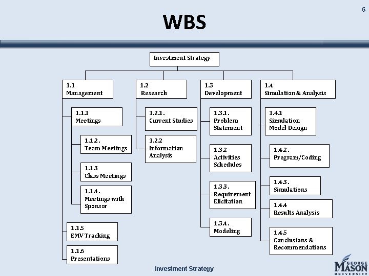
6 WBS Investment Strategy 1. 1 Management 1. 1. 1 Meetings 1. 1. 2. Team Meetings 1. 1. 3 Class Meetings 1. 1. 4. Meetings with Sponsor 1. 1. 5 EMV Tracking 1. 2 Research 1. 2. 1. Current Studies 1. 2. 2 Information Analysis 1. 3 Development 1. 3. 1. Problem Statement 1. 3. 2 Activities Schedules 1. 3. 3. Requirement Elicitation 1. 3. 4. Modeling 1. 1. 6 Presentations Investment Strategy 1. 4 Simulation & Analysis 1. 4. 1 Simulation Model Design 1. 4. 2. Program/Coding 1. 4. 3. Simulations 1. 4. 4 Results Analysis 1. 4. 5 Conclusions & Recommendations

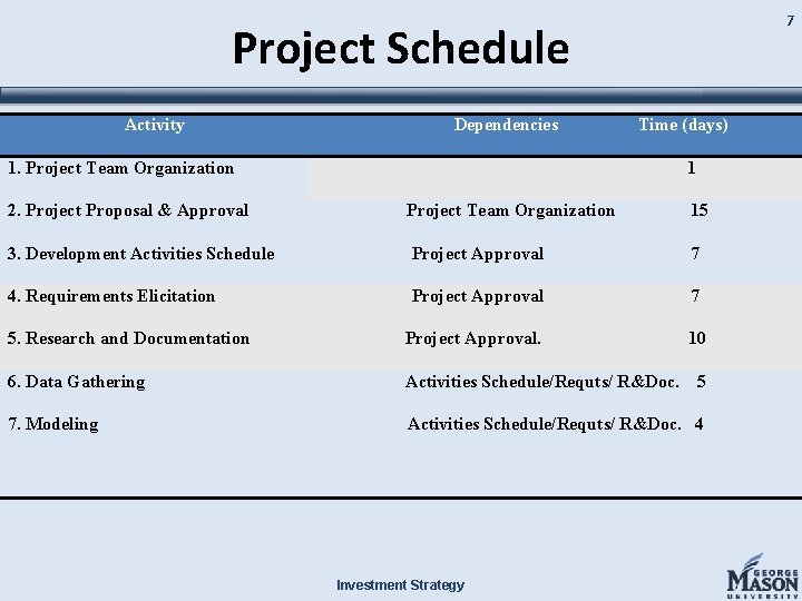
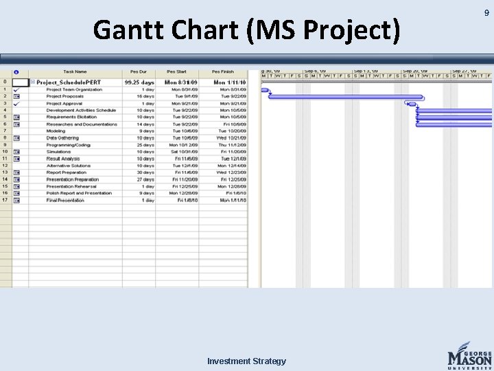
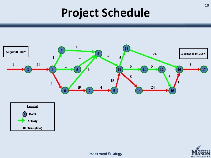
7 Project Schedule Activity Dependencies Time (days) 1. Project Team Organization 1 2. Project Proposal & Approval Project Team Organization 15 3. Development Activities Schedule Project Approval 7 4. Requirements Elicitation Project Approval 7 5. Research and Documentation Project Approval. 10 6. Data Gathering Activities Schedule/Requts/ R&Doc. 7. Modeling Activities Schedule/Requts/ R&Doc. 4 Investment Strategy 5

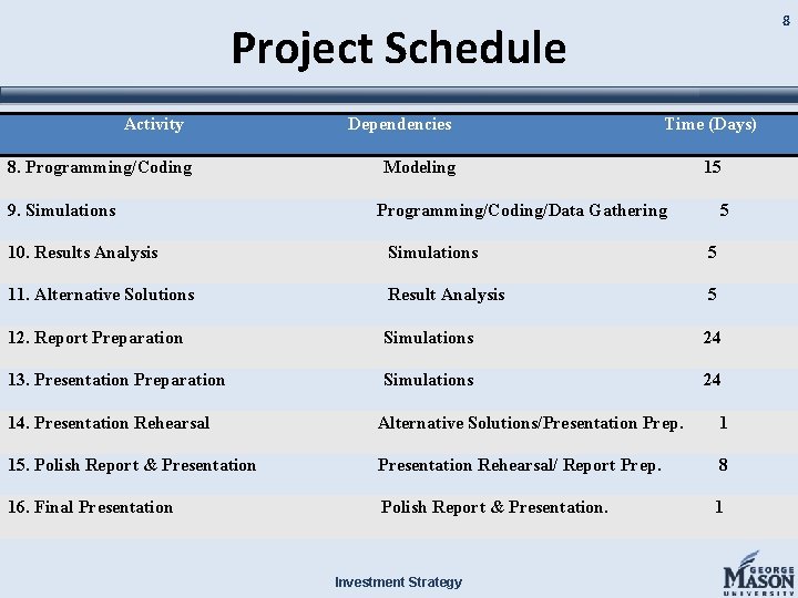
8 Project Schedule Activity 8. Programming/Coding 9. Simulations Dependencies Time (Days) Modeling 15 Programming/Coding/Data Gathering 5 10. Results Analysis Simulations 5 11. Alternative Solutions Result Analysis 5 12. Report Preparation Simulations 24 13. Presentation Preparation Simulations 24 14. Presentation Rehearsal Alternative Solutions/Presentation Prep. 1 15. Polish Report & Presentation Rehearsal/ Report Prep. 8 16. Final Presentation Polish Report & Presentation. 1 Investment Strategy

Gantt Chart (MS Project) Investment Strategy 9

10 Project Schedule 7 4 August 31, 2009 13 8 1 1 14 2 3 5 7 1 5 5 10 10 15 1 6 10 7 4 9 Legend 2 Event Activity 10 Time (days) Investment Strategy December 18, 2009 24 5 11 5 5 8 12 16 5 1 14 24 15 17

EVM Investment Strategy 11

CPI Investment Strategy 12

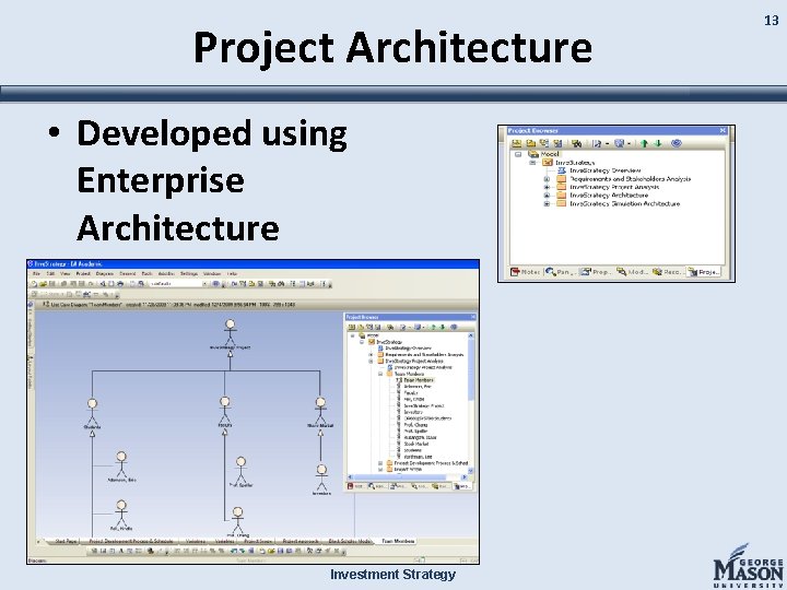
Project Architecture • Developed using Enterprise Architecture Investment Strategy 13

Related Research • “Expected Option Returns” by Joshua D. Coval and Tyler Shumway Univ. of Michigan Business School, June 2000 – Examined expected option returns of straddle strategy based on S&P 500 – Results indicated sellers can expect an average gain of 3% per week Investment Strategy 14

Definition of Terms (1) • Put – A put option gives the holder the right, but not the obligation, to sell the underlying asset by a certain date for a certain price • Call – A call option gives the holder the right, but not the obligation, to buy the underlying asset by a certain date for a certain price Investment Strategy 15

Definition of Terms (2) • Strike Price – the fixed price at which the owner of an option can exercise (buy or sell) the underlying derivative before the expiration date • Volatility – a quantitative value indicating the uncertainty and risk of the underlying asset over time Investment Strategy 16

Definition of Terms (3) • European Option – may only be exercised at the expiration date • American Option – may be exercised at any time before the expiration date • Black Scholes Formula – A mathematical formula used to obtain the price of put and call options Investment Strategy 17

Definition of Terms (4) • Stop Loss – the maximum amount of loss a seller is willing to accept before buying back an option • Time Value Decay – the loss of value of an option as it moves towards expiration Investment Strategy 18

Definition of Terms (5) • Straddle Strategy – simultaneously selling a put and call at the money • Strangle Strategy – simultaneously selling a put and a call out of the money – Symmetric strike prices (+-10, +-20, etc. ) – Asymmetric Investment Strategy 19

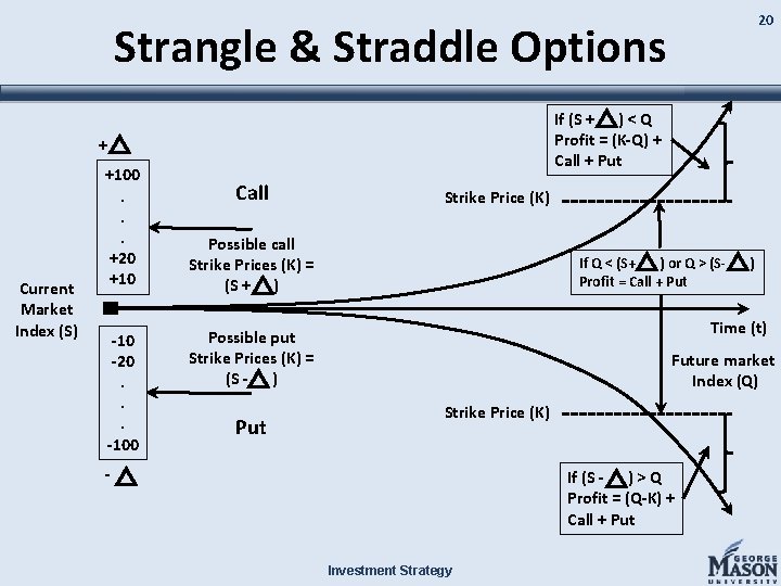
20 Strangle & Straddle Options If (S + ) < Q Profit = (K-Q) + Call + Put + Current Market Index (S) +100. . . +20 +10 -20. . . -100 Call Strike Price (K) Possible call Strike Prices (K) = (S + ) If Q < (S+ ) or Q > (SProfit = Call + Put Time (t) Possible put Strike Prices (K) = (S - ) Put ) Future market Index (Q) Strike Price (K) - If (S - ) > Q Profit = (Q-K) + Call + Put Investment Strategy

Scope • • S&P 500 American Options 9 years historical data 45 day trading period beginning on third Friday of previous month Investment Strategy 21

Requirements Our project: 1. Shall incorporate 9 years of historical S&P 500, CBOE VIX and LIBOR Rate data 2. Should identify the most successful strategy for each day in the investment period 3. Should determine the expected monthly return for a seller for a given strategy Investment Strategy 22

Problem Approach • Determine strategy • Develop simulation • Refine simulation iteratively – based on sponsor feedback • Analyze Results Investment Strategy 23

Simulation • Uses Matlab – Over 5 million profit calculations • Calculates option price for put and call for each day in 45 day trading window over a 9 year period • Produces monthly and yearly profit averages • Determines most profitable investment strategy for each day in 45 day period Investment Strategy 24

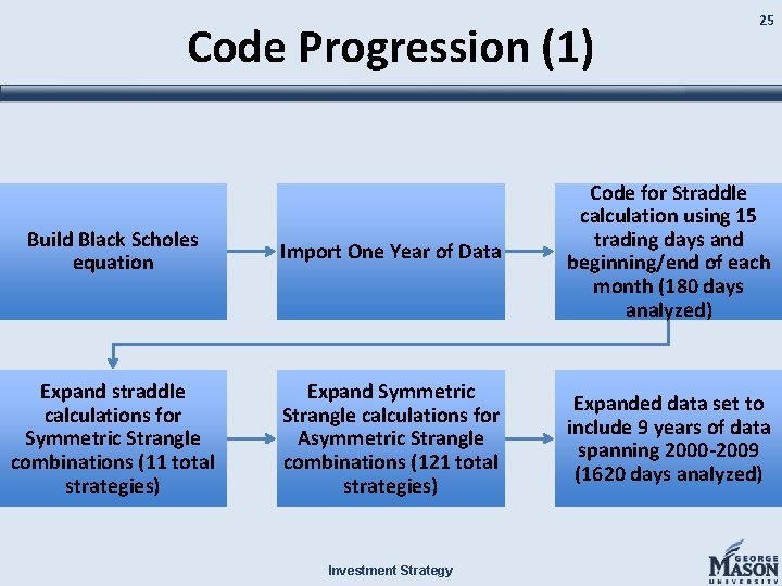
Code Progression (1) 25 Build Black Scholes equation Import One Year of Data Code for Straddle calculation using 15 trading days and beginning/end of each month (180 days analyzed) Expand straddle calculations for Symmetric Strangle combinations (11 total strategies) Expand Symmetric Strangle calculations for Asymmetric Strangle combinations (121 total strategies) Expanded data set to include 9 years of data spanning 2000 -2009 (1620 days analyzed) Investment Strategy

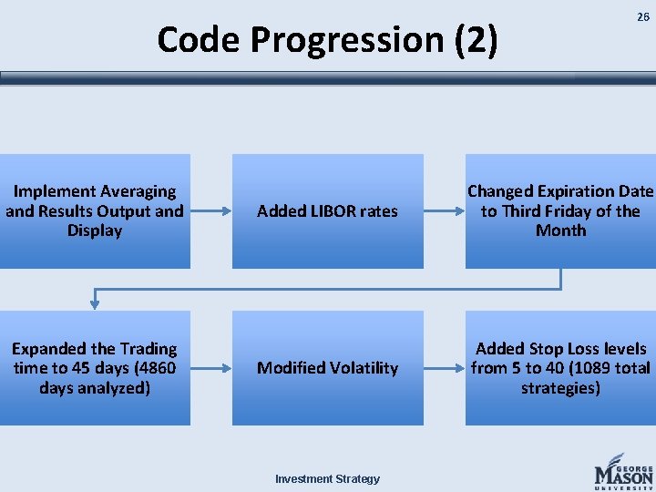
Code Progression (2) Implement Averaging and Results Output and Display Expanded the Trading time to 45 days (4860 days analyzed) 26 Added LIBOR rates Changed Expiration Date to Third Friday of the Month Modified Volatility Added Stop Loss levels from 5 to 40 (1089 total strategies) Investment Strategy

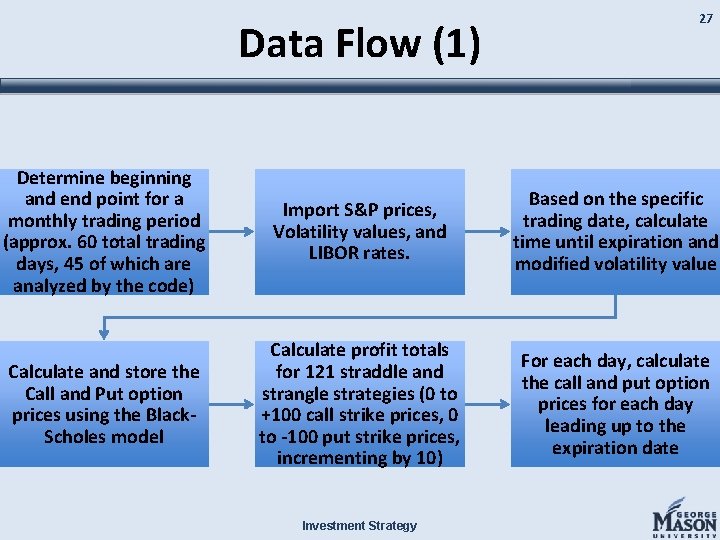
Data Flow (1) 27 Determine beginning and end point for a monthly trading period (approx. 60 total trading days, 45 of which are analyzed by the code) Import S&P prices, Volatility values, and LIBOR rates. Based on the specific trading date, calculate time until expiration and modified volatility value Calculate and store the Call and Put option prices using the Black. Scholes model Calculate profit totals for 121 straddle and strangle strategies (0 to +100 call strike prices, 0 to -100 put strike prices, incrementing by 10) For each day, calculate the call and put option prices for each day leading up to the expiration date Investment Strategy

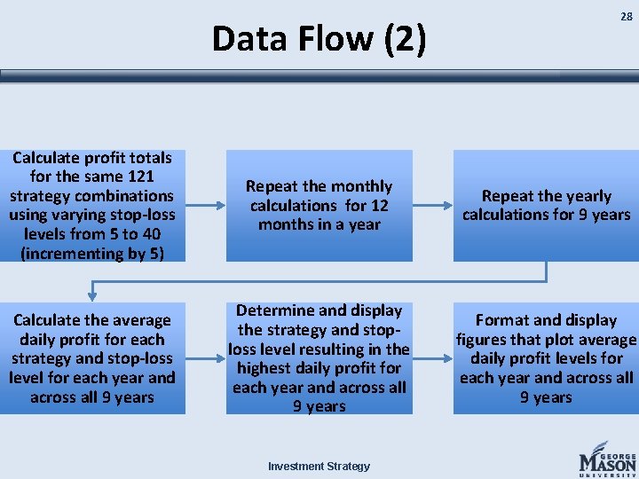
Data Flow (2) 28 Calculate profit totals for the same 121 strategy combinations using varying stop-loss levels from 5 to 40 (incrementing by 5) Repeat the monthly calculations for 12 months in a year Repeat the yearly calculations for 9 years Calculate the average daily profit for each strategy and stop-loss level for each year and across all 9 years Determine and display the strategy and stoploss level resulting in the highest daily profit for each year and across all 9 years Format and display figures that plot average daily profit levels for each year and across all 9 years Investment Strategy

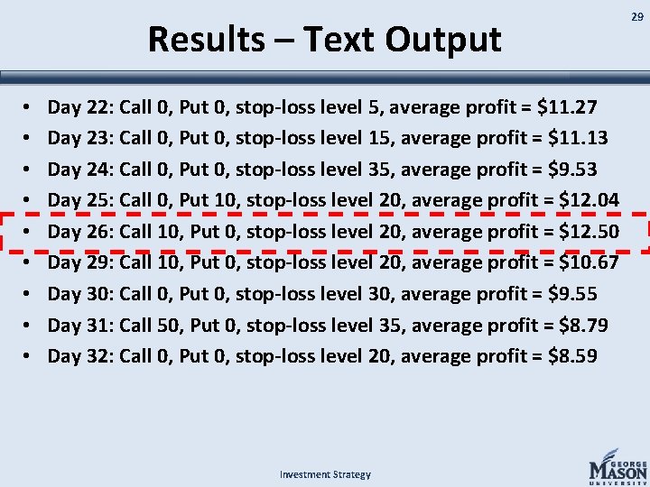
Results – Text Output • • • Day 22: Call 0, Put 0, stop-loss level 5, average profit = $11. 27 Day 23: Call 0, Put 0, stop-loss level 15, average profit = $11. 13 Day 24: Call 0, Put 0, stop-loss level 35, average profit = $9. 53 Day 25: Call 0, Put 10, stop-loss level 20, average profit = $12. 04 Day 26: Call 10, Put 0, stop-loss level 20, average profit = $12. 50 Day 29: Call 10, Put 0, stop-loss level 20, average profit = $10. 67 Day 30: Call 0, Put 0, stop-loss level 30, average profit = $9. 55 Day 31: Call 50, Put 0, stop-loss level 35, average profit = $8. 79 Day 32: Call 0, Put 0, stop-loss level 20, average profit = $8. 59 Investment Strategy 29

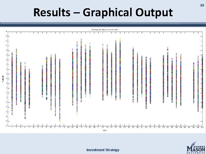
Results – Graphical Output Investment Strategy 30

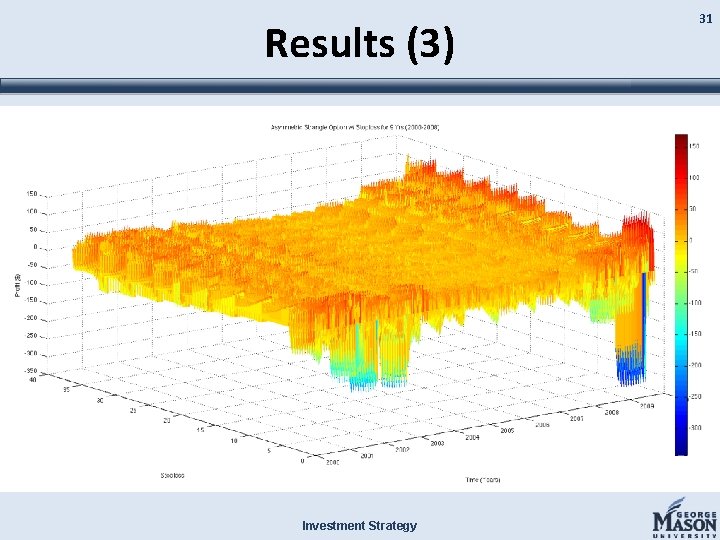
Results (3) Investment Strategy 31

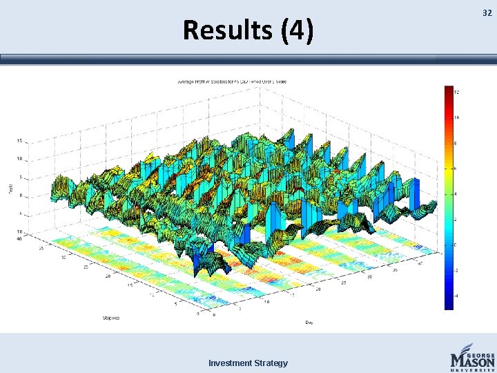
Results (4) Investment Strategy 32

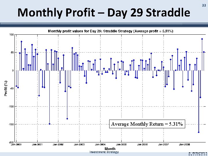
Monthly Profit – Day 29 Straddle Average Monthly Return = 5. 31% Investment Strategy 33

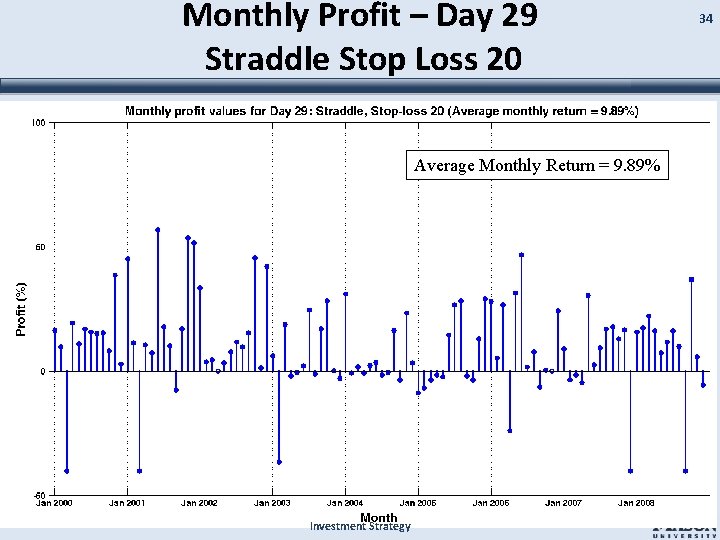
Monthly Profit – Day 29 Straddle Stop Loss 20 Average Monthly Return = 9. 89% Investment Strategy 34

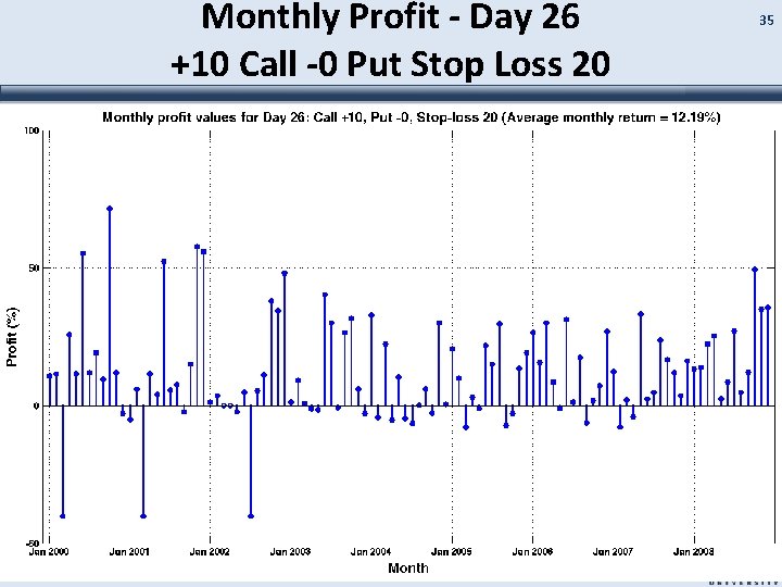
Monthly Profit - Day 26 +10 Call -0 Put Stop Loss 20 Average Monthly Return = 12. 19% Investment Strategy 35

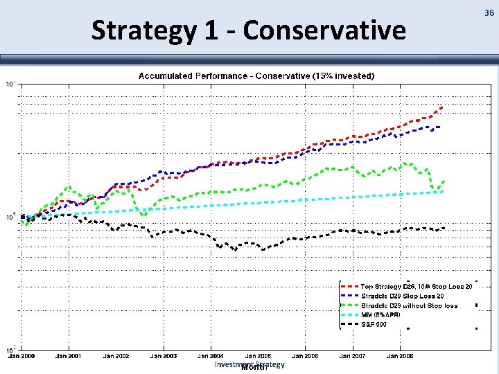
Strategy 1 - Conservative Investment Strategy 36

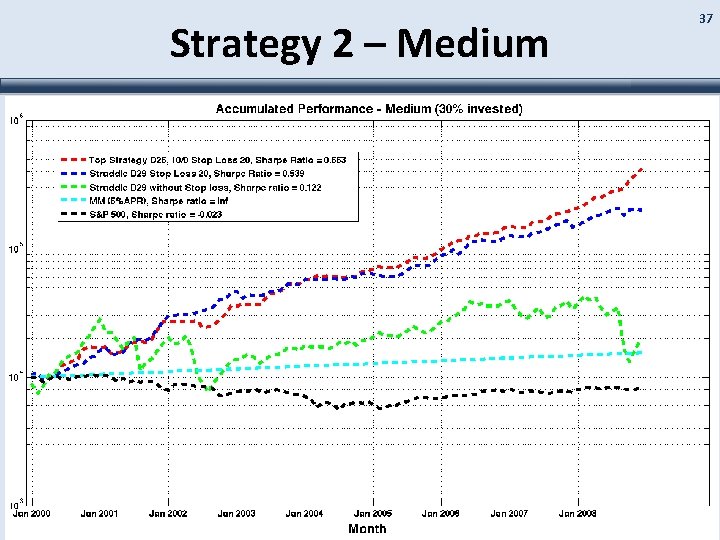
Strategy 2 – Medium Investment Strategy 37

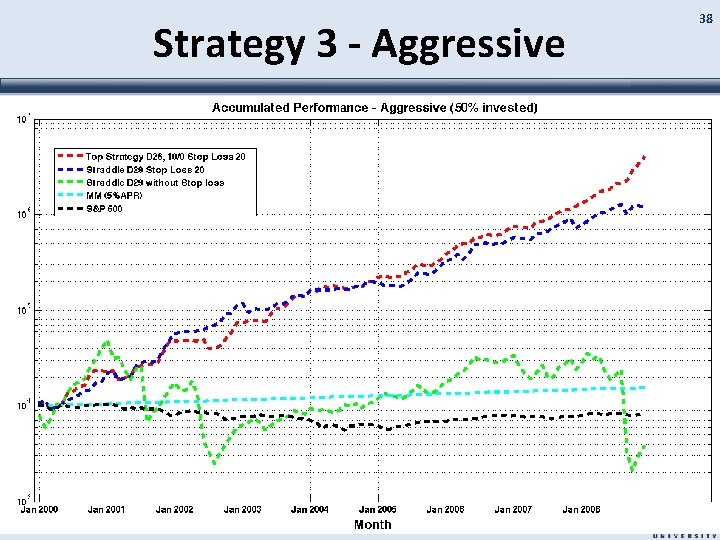
Strategy 3 - Aggressive Investment Strategy 38

Verification of Results • Wrote code to calculate the average rate of return (Ro. R) for each week over 9 years – Ro. R = profit/premium • Results indicate average Ro. R of ~2% per week • Consistent with previous research Investment Strategy 39

Future Research • Expand simulation to incorporate other investment strategies • Obtain actual market data to use in simulation ($$) • Modify Black Scholes formula to be more accurate – Solve for volatility • Adjust strategy to buy back option after stop loss condition Investment Strategy 40

Business Possibilities • • Strategy Consultants Investment Firm Productize (software) License Algorithm Investment Strategy 41

Project Website • http: //mason. gmu. edu/~lvorthma – Deliverables – Code – Data files – Related Research Papers – Project schedule Investment Strategy 42

Questions? Investment Strategy

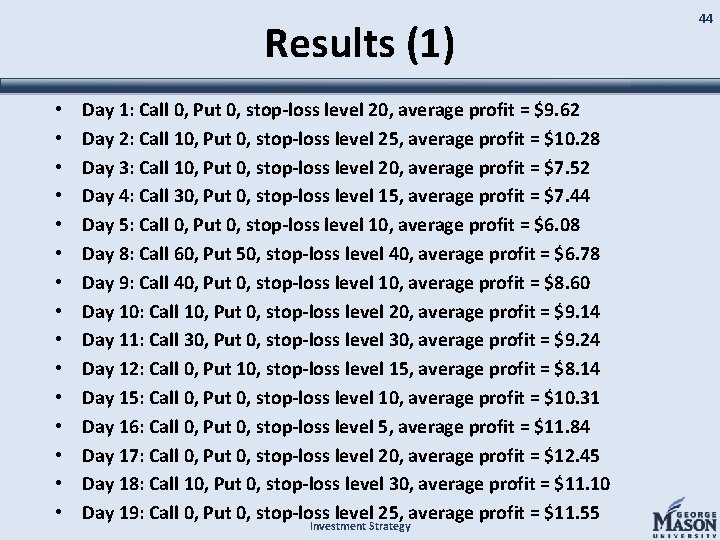
Results (1) • • • • Day 1: Call 0, Put 0, stop-loss level 20, average profit = $9. 62 Day 2: Call 10, Put 0, stop-loss level 25, average profit = $10. 28 Day 3: Call 10, Put 0, stop-loss level 20, average profit = $7. 52 Day 4: Call 30, Put 0, stop-loss level 15, average profit = $7. 44 Day 5: Call 0, Put 0, stop-loss level 10, average profit = $6. 08 Day 8: Call 60, Put 50, stop-loss level 40, average profit = $6. 78 Day 9: Call 40, Put 0, stop-loss level 10, average profit = $8. 60 Day 10: Call 10, Put 0, stop-loss level 20, average profit = $9. 14 Day 11: Call 30, Put 0, stop-loss level 30, average profit = $9. 24 Day 12: Call 0, Put 10, stop-loss level 15, average profit = $8. 14 Day 15: Call 0, Put 0, stop-loss level 10, average profit = $10. 31 Day 16: Call 0, Put 0, stop-loss level 5, average profit = $11. 84 Day 17: Call 0, Put 0, stop-loss level 20, average profit = $12. 45 Day 18: Call 10, Put 0, stop-loss level 30, average profit = $11. 10 Day 19: Call 0, Put 0, stop-loss level 25, average profit = $11. 55 Investment Strategy 44

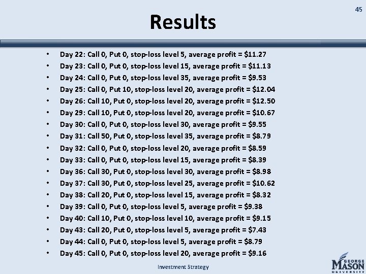
Results • • • • • Day 22: Call 0, Put 0, stop-loss level 5, average profit = $11. 27 Day 23: Call 0, Put 0, stop-loss level 15, average profit = $11. 13 Day 24: Call 0, Put 0, stop-loss level 35, average profit = $9. 53 Day 25: Call 0, Put 10, stop-loss level 20, average profit = $12. 04 Day 26: Call 10, Put 0, stop-loss level 20, average profit = $12. 50 Day 29: Call 10, Put 0, stop-loss level 20, average profit = $10. 67 Day 30: Call 0, Put 0, stop-loss level 30, average profit = $9. 55 Day 31: Call 50, Put 0, stop-loss level 35, average profit = $8. 79 Day 32: Call 0, Put 0, stop-loss level 20, average profit = $8. 59 Day 33: Call 0, Put 0, stop-loss level 15, average profit = $8. 39 Day 36: Call 30, Put 0, stop-loss level 30, average profit = $8. 98 Day 37: Call 30, Put 0, stop-loss level 25, average profit = $10. 62 Day 38: Call 20, Put 0, stop-loss level 15, average profit = $8. 32 Day 39: Call 0, Put 0, stop-loss level 5, average profit = $9. 38 Day 40: Call 10, Put 0, stop-loss level 10, average profit = $9. 15 Day 43: Call 20, Put 0, stop-loss level 5, average profit = $7. 43 Day 44: Call 0, Put 0, stop-loss level 5, average profit = $8. 79 Day 45: Call 0, Put 0, stop-loss level 20, average profit = $9. 16 Investment Strategy 45