INVESTIGATION Data Colllection Data Presentation Tabulation Diagrams Graphs

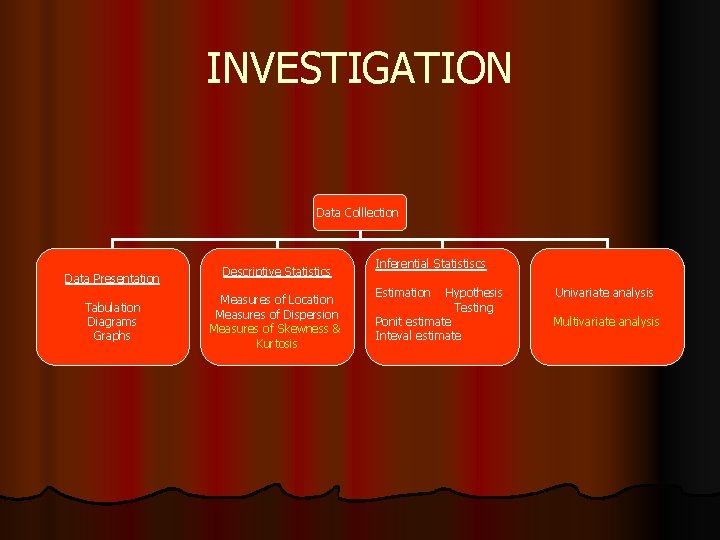
INVESTIGATION Data Colllection Data Presentation Tabulation Diagrams Graphs Descriptive Statistics Measures of Location Measures of Dispersion Measures of Skewness & Kurtosis Inferential Statistiscs Estimation Hypothesis Testing Ponit estimate Inteval estimate Univariate analysis Multivariate analysis

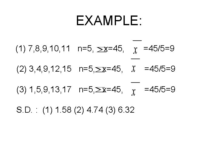
EXAMPLE: (1) 7, 8, 9, 10, 11 n=5, x=45, =45/5=9 (2) 3, 4, 9, 12, 15 n=5, x=45, =45/5=9 (3) 1, 5, 9, 13, 17 n=5, x=45, =45/5=9 S. D. : (1) 1. 58 (2) 4. 74 (3) 6. 32

Measures of Dispersion Or Measures of variability 3

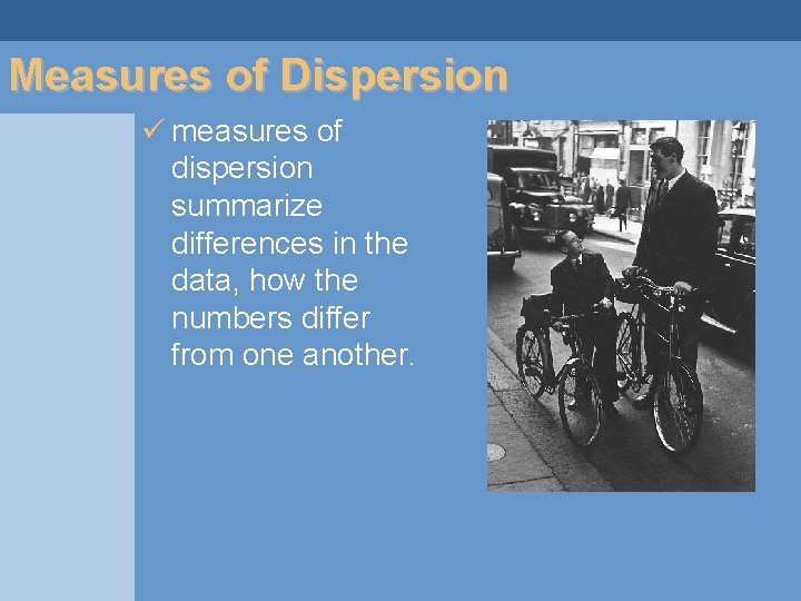
Measures of Dispersion ü measures of dispersion summarize differences in the data, how the numbers differ from one another.

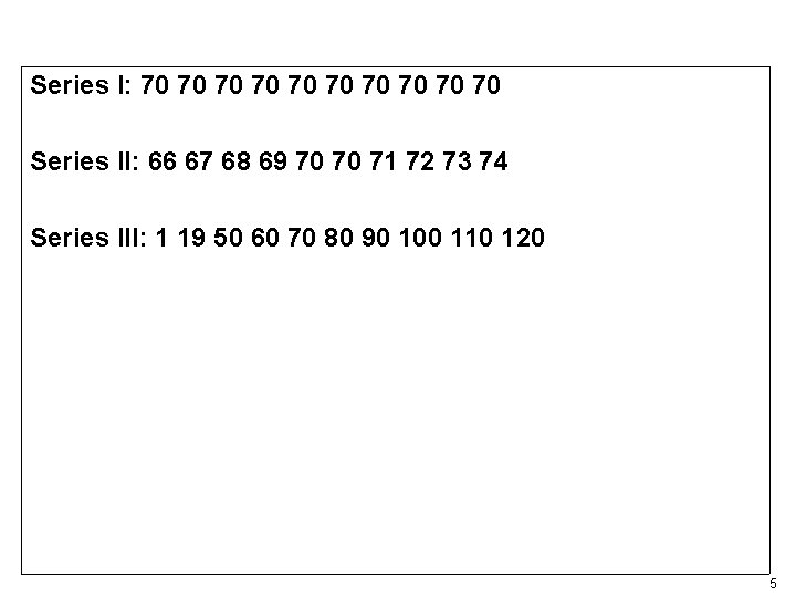
Series I: 70 70 70 Series II: 66 67 68 69 70 70 71 72 73 74 Series III: 1 19 50 60 70 80 90 100 110 120 5

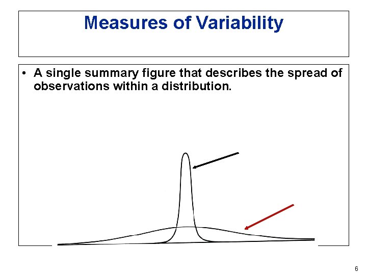
Measures of Variability • A single summary figure that describes the spread of observations within a distribution. 6

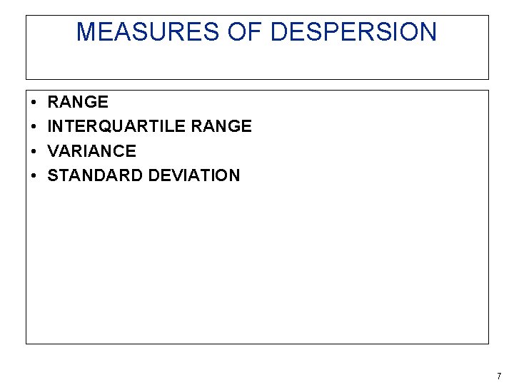
MEASURES OF DESPERSION • • RANGE INTERQUARTILE RANGE VARIANCE STANDARD DEVIATION 7

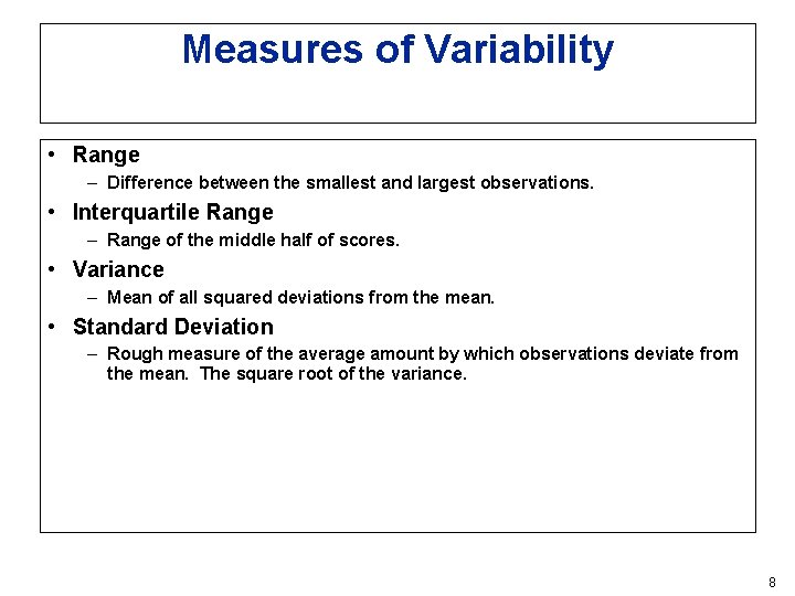
Measures of Variability • Range – Difference between the smallest and largest observations. • Interquartile Range – Range of the middle half of scores. • Variance – Mean of all squared deviations from the mean. • Standard Deviation – Rough measure of the average amount by which observations deviate from the mean. The square root of the variance. 8

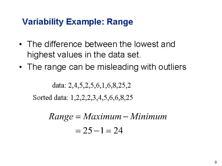
Variability Example: Range • The difference between the lowest and highest values in the data set. • The range can be misleading with outliers data: 2, 4, 5, 2, 5, 6, 1, 6, 8, 25, 2 Sorted data: 1, 2, 2, 2, 3, 4, 5, 6, 6, 8, 25 9

Measures of Position Quartiles, Deciles, Percentiles 10

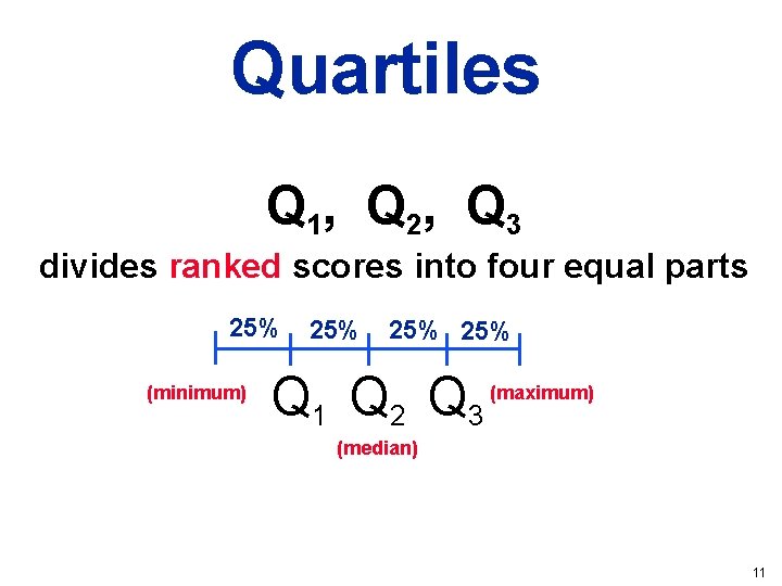
Quartiles Q 1, Q 2, Q 3 divides ranked scores into four equal parts 25% (minimum) 25% 25% Q 1 Q 2 Q 3 (maximum) (median) 11

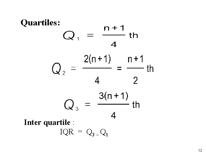
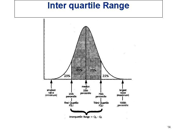
Quartiles: Inter quartile : IQR = Q 3 – Q 1 12

Inter quartile Range • The inter quartile range is Q 3 -Q 1 • 50% of the observations in the distribution are in the inter quartile range. • The following figure shows the interaction between the quartiles, the median and the inter quartile range. 13

Inter quartile Range 14

Sample Number Unsorted Values 1 25 2 27 3 20 4 23 5 26 6 24 7 19 8 16 9 25 10 18 11 30 12 29 13 32 14 26 15 24 16 21 17 28 18 27 19 20 20 16 21 14 15

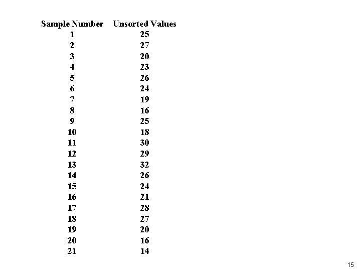
Sample Number Unsorted Values 1 25 2 27 3 20 4 23 5 26 6 24 7 19 8 16 9 25 10 18 11 30 12 29 13 32 14 26 15 24 16 21 17 28 18 27 19 20 20 16 21 14 Ranked Values 14 16 16 18 19 20 20 21 23 24 24 25 25 26 26 27 27 28 29 30 32 16

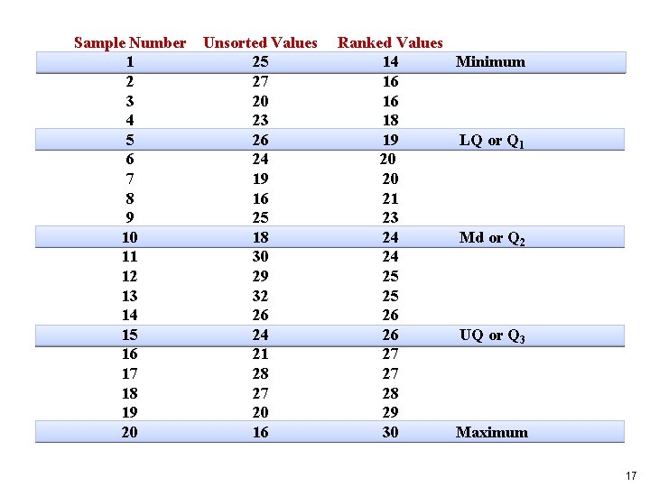
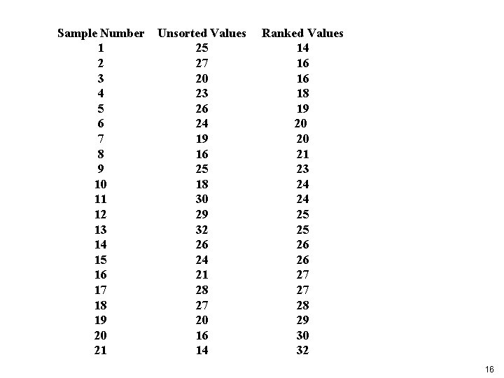
Sample Number Unsorted Values 1 25 2 27 3 20 4 23 5 26 6 24 7 19 8 16 9 25 10 18 11 30 12 29 13 32 14 26 15 24 16 21 17 28 18 27 19 20 20 16 Ranked Values 14 Minimum 16 16 18 19 LQ or Q 1 20 20 21 23 24 Md or Q 2 24 25 25 26 26 UQ or Q 3 27 27 28 29 30 Maximum 17

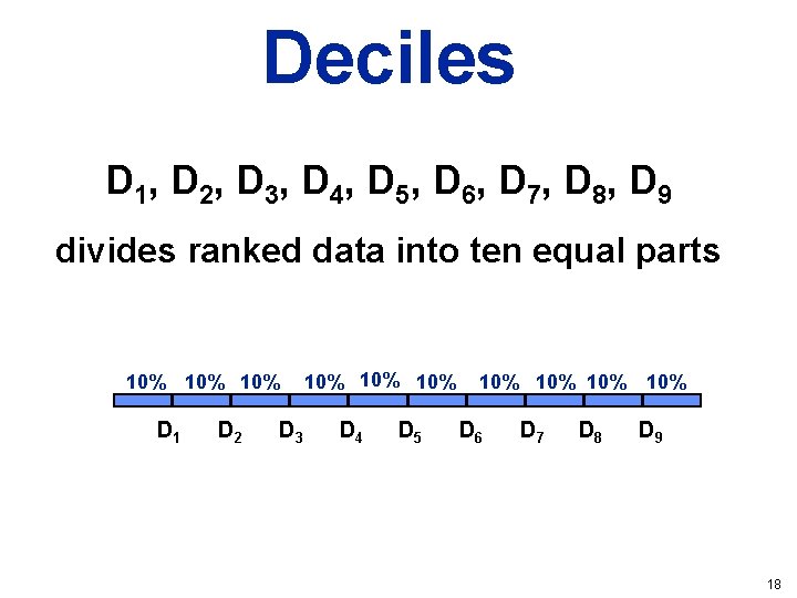
Deciles D 1, D 2, D 3, D 4, D 5, D 6, D 7, D 8, D 9 divides ranked data into ten equal parts 10% 10% D 1 D 2 D 3 10% 10% D 4 D 5 10% 10% D 6 D 7 D 8 D 9 18

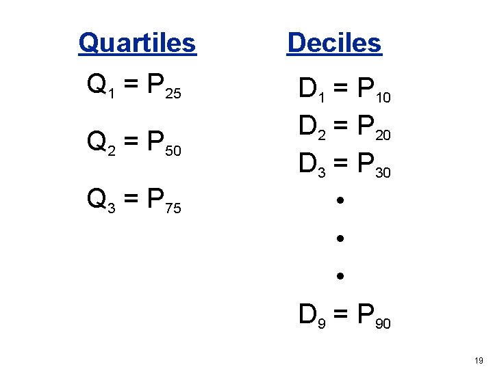
Quartiles Q 1 = P 25 Q 2 = P 50 Q 3 = P 75 Deciles D 1 = P 10 D 2 = P 20 D 3 = P 30 • • • D 9 = P 90 19

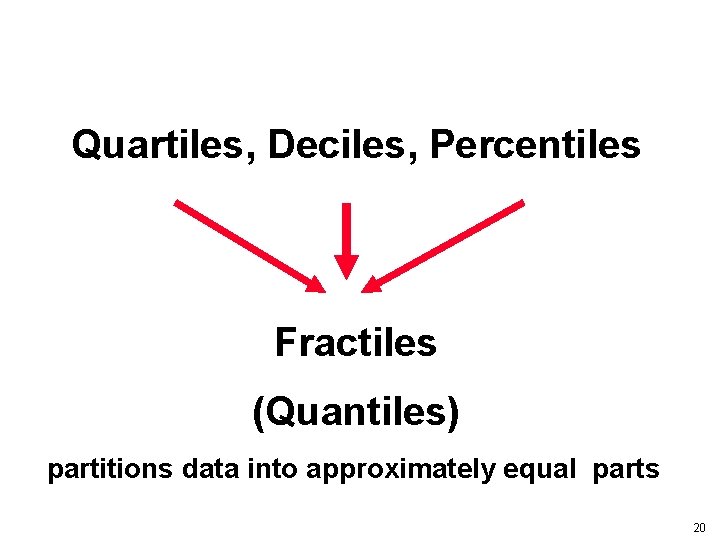
Quartiles, Deciles, Percentiles Fractiles (Quantiles) partitions data into approximately equal parts 20

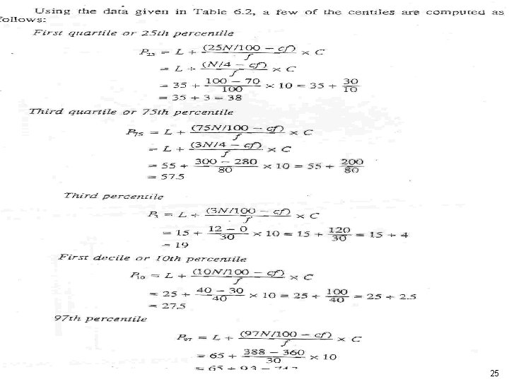
Percentiles and Quartiles • Maximum is 100 th percentile: 100% of values lie at or below the maximum • Median is 50 th percentile: 50% of values lie at or below the median • Any percentile can be calculated. But the most common are 25 th (1 st Quartile) and 75 th (3 rd Quartile) 21

Locating Percentiles in a Frequency Distribution • A percentile is a score below which a specific percentage of the distribution falls(the median is the 50 th percentile. • The 75 th percentile is a score below which 75% of the cases fall. • The median is the 50 th percentile: 50% of the cases fall below it • Another type of percentile : The quartile lower quartile is 25 th percentile and the upper quartile is the 75 th percentile 22

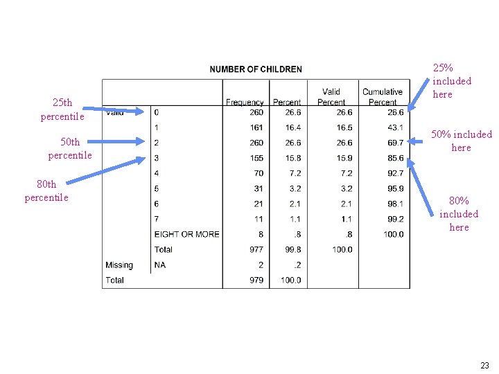
25 th percentile 50 th percentile 80 th percentile 25% included here 50% included here 80% included here 23

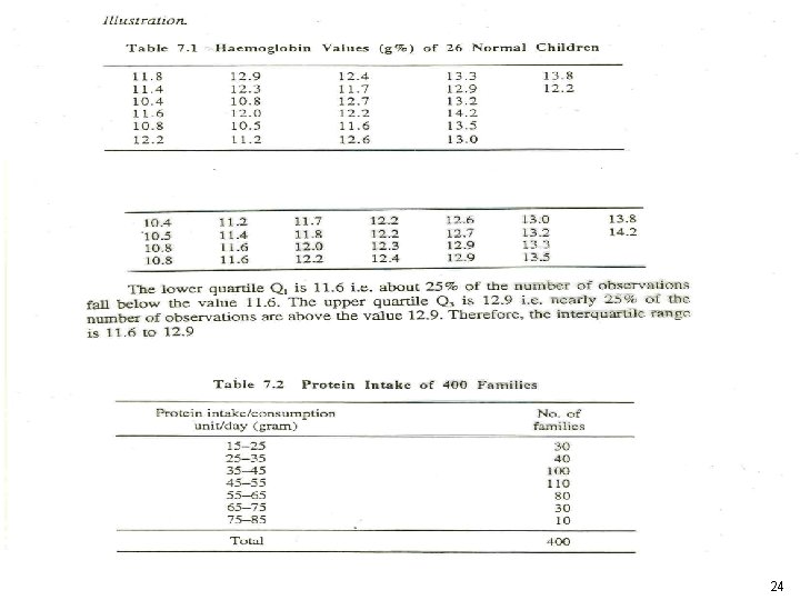
24

25

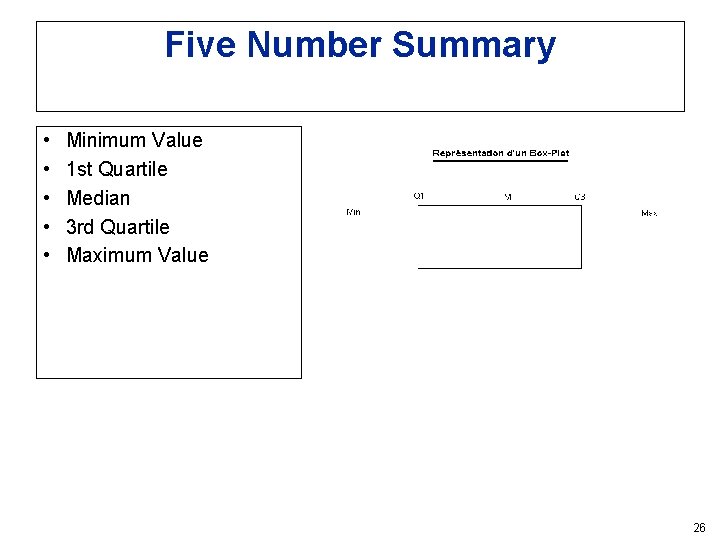
Five Number Summary • • • Minimum Value 1 st Quartile Median 3 rd Quartile Maximum Value 26

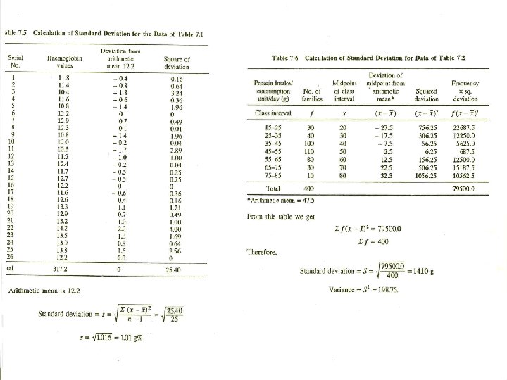
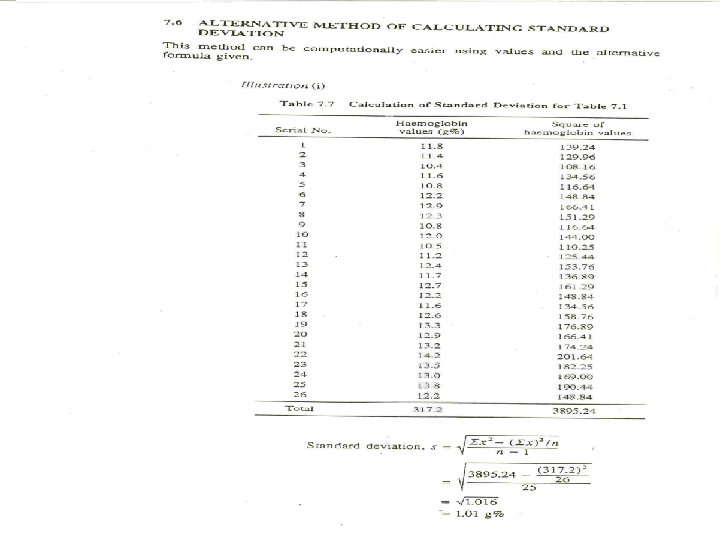
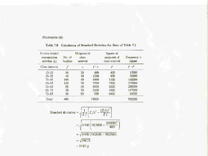
VARIANCE: Deviations of each observation from the mean, then averaging the sum of squares of these deviations. STANDARD DEVIATION: “ ROOT- MEANS-SQUARE-DEVIATIONS” 27

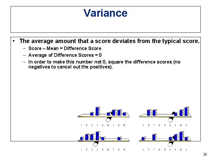
Variance • The average amount that a score deviates from the typical score. – Score – Mean = Difference Score – Average of Difference Scores = 0 – In order to make this number not 0, square the difference scores (no negatives to cancel out the positives). 28

Standard Deviation • To “undo” the squaring of difference scores, take the square root of the variance. • Return to original units rather than squared units. 29

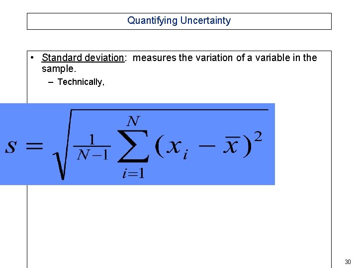
Quantifying Uncertainty • Standard deviation: measures the variation of a variable in the sample. – Technically, 30

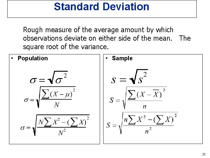
Standard Deviation Rough measure of the average amount by which observations deviate on either side of the mean. The square root of the variance. • Population • Sample 31

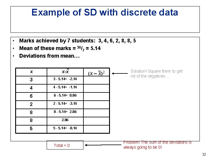
Example of SD with discrete data • Marks achieved by 7 students: 3, 4, 6, 2, 8, 8, 5 • Mean of these marks = 36/7 = 5. 14 • Deviations from mean… x x-x 3 3 - 5. 14= -2. 14 4 4 - 5. 14= -1. 14 6 6 - 5. 14= 0. 86 2 2 - 5. 14= -3. 14 8 8 - 5. 14= 2. 86 8 2. 86 5 5 - 5. 14= -0. 14 Total = 0 (x – x)2 Solution! Square them to get rid of the negatives… Problem! The sum of the deviations is always going to be 0! 32

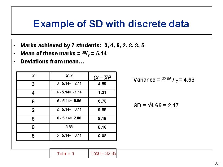
Example of SD with discrete data • Marks achieved by 7 students: 3, 4, 6, 2, 8, 8, 5 • Mean of these marks = 36/7 = 5. 14 • Deviations from mean… x x-x (x – x)2 3 3 - 5. 14= -2. 14 4. 59 4 4 - 5. 14= -1. 14 1. 31 6 6 - 5. 14= 0. 86 0. 73 2 2 - 5. 14= -3. 14 9. 88 8 8 - 5. 14= 2. 86 8. 16 8 2. 86 8. 16 5 5 - 5. 14= -0. 14 0. 02 Total = 0 Variance = 32. 85 / 7 = 4. 69 SD = √ 4. 69 = 2. 17 Total = 32. 85 33

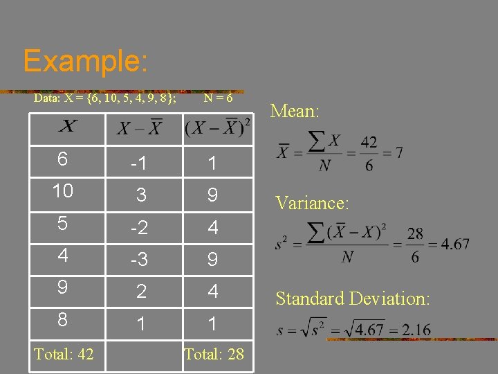
Example: Data: X = {6, 10, 5, 4, 9, 8}; N=6 6 -1 1 10 3 9 5 -2 4 4 -3 9 9 2 4 8 1 1 Total: 42 Total: 28 Mean: Variance: Standard Deviation:

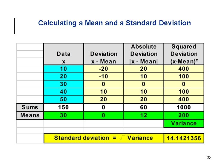
Calculating a Mean and a Standard Deviation 35

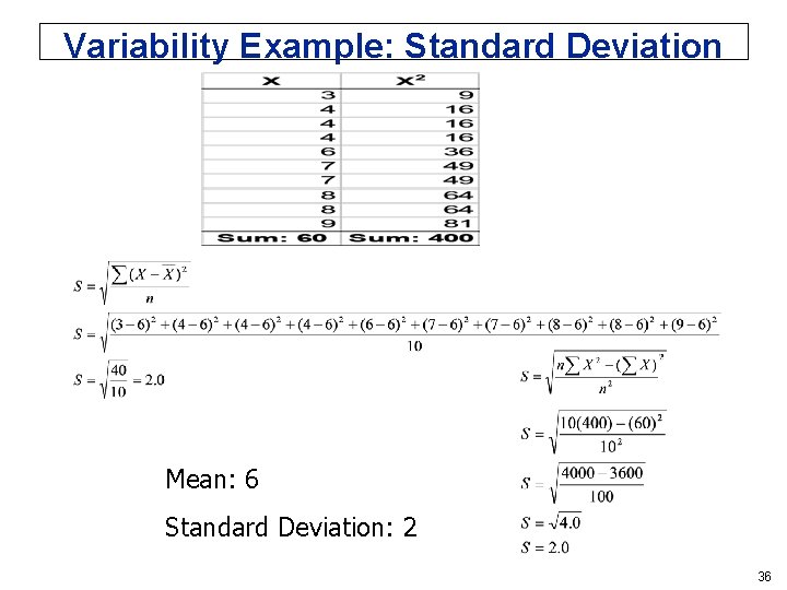
Variability Example: Standard Deviation Mean: 6 Standard Deviation: 2 36

37

38

39

Mean and Standard Deviation • Using the mean and standard deviation together: – Is an efficient way to describe a distribution with just two numbers. – Allows a direct comparison between distributions that are on different scales. 40

WHICH MEASURE TO USE ? DISTRIBUTION OF DATA IS SYMMETRIC ---- USE MEAN & S. D. , DISTRIBUTION OF DATA IS SKEWED ---- USE MEDIAN & QUARTILES 41

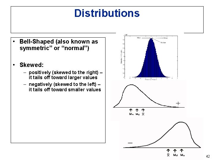
Distributions • Bell-Shaped (also known as symmetric” or “normal”) • Skewed: – positively (skewed to the right) – it tails off toward larger values – negatively (skewed to the left) – it tails off toward smaller values 42

43

ANY QUESTIONS 44