Inventory Models Inventory n Any stored resource used

Inventory Models

Inventory n Any stored resource used to satisfy a current or future need (raw materials, work-in-process, finished goods, etc. ) n Represents as much as 50% of invested capitol at some companies n Excessive inventory levels are

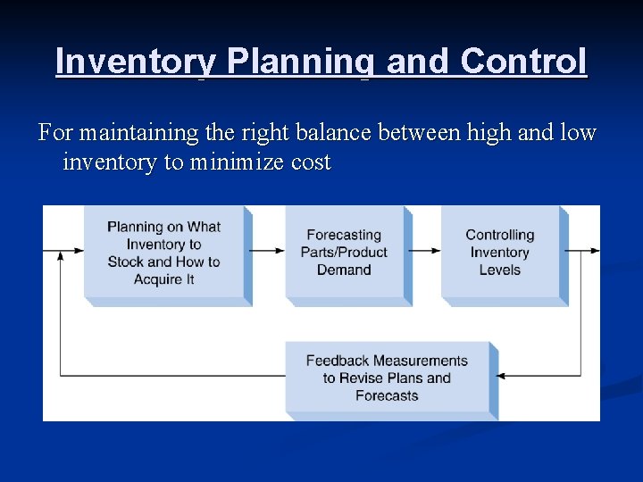
Inventory Planning and Control For maintaining the right balance between high and low inventory to minimize cost

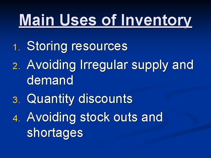
Main Uses of Inventory 1. 2. 3. 4. Storing resources Avoiding Irregular supply and demand Quantity discounts Avoiding stock outs and shortages

Inventory Control Decisions Objective: Minimize total inventory cost by controlling ordering cost & the inventory carrying cost Decisions: n How much to order? n When to order?

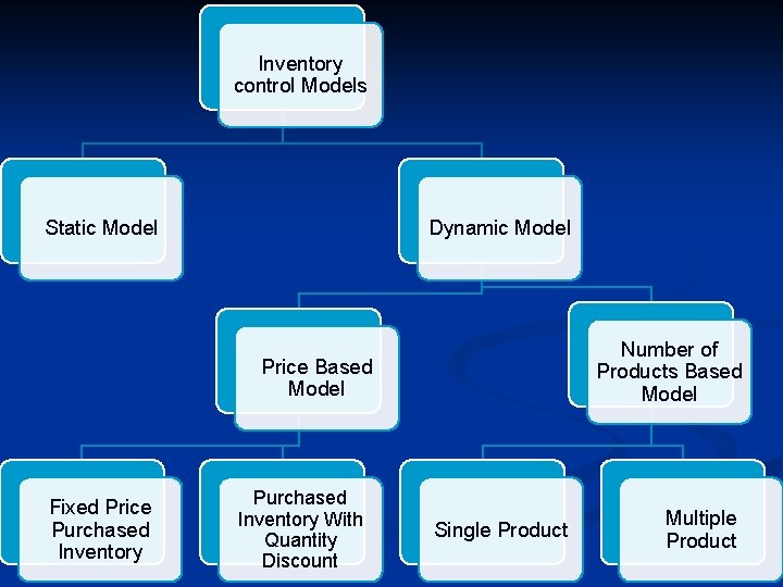
Inventory control Models Static Model Dynamic Model Number of Products Based Model Price Based Model Fixed Price Purchased Inventory With Quantity Discount Single Product Multiple Product

Inventory Models n Help to decide n. How much to order n. When n Basic n POQ to order EOQ model

STATIC MODEL

Independent Demand Inventory Models-I n Introduction The average manufacturing company spends over onehalf of its sales revenue on inventory. Because of the large investment and expenditure required for acquiring and controlling inventories and their effect on profits, successful companies devote a great deal of attention to inventory management. n How much inventory is enough? - Marketing department wants large inventory, it does not like stock outs. - Finance department likes low inventory and high turnover to minimize funds tied up in inventories; opportunity cost of capital. 1 - 9 Introduction

Single Period Model n Single period model: model for ordering of perishables and other items with limited useful lives n Shortage cost: generally the unrealized profits per unit n Excess cost: difference between purchase cost and salvage value of items left over at the end of a period 12 -10

Single Period Model n n 12 -11 Continuous stocking levels n Identifies optimal stocking levels n Optimal stocking level balances unit shortage and excess cost Discrete stocking levels n Service levels are discrete rather than continuous n Desired service level is equaled or exceeded

n Demand - certainty - risk, probability distribution of demand - uncertainty, nothing known n Lead time: The period between the order time and the delivery time - certainty - risk, probability distribution of demand - uncertainty n Inside or Outside Procurement - purchased from outside; pure inventory problem - integrated with production smoothing if inside 1 - 12 Introduction

Single Period Stochastic Inventory Models These models have the objective of properly balancing the cost of Underage – having not ordered enough products vs. Overage – having ordered more than we can sell n These models apply to problems like: n Planning initial shipments of ‘High-Fashion’ items n Amount of perishable food products n Item with short shelf life (like the daily n

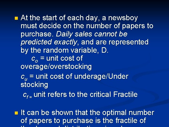
n At the start of each day, a newsboy must decide on the number of papers to purchase. Daily sales cannot be predicted exactly, and are represented by the random variable, D. co = unit cost of overage/overstocking cu = unit cost of underage/Under stocking cf = unit refers to the critical Fractile n It can be shown that the optimal number of papers to purchase is the fractile of

n Assuming we have a certain number of parts on hand, u > 0 n This is true only if the product under study has a shelf life that extends beyond one period n Here we still compute Q* will order only Q* - u (or 0 if u > Q*)

DYNAMIC MODELS

General Framework for Inventory Models-II n Static and Dynamic Problems - Static: one period problem, classic examples are - Dynamic: decisions over time n Behavior of Demand through Time and for Various Items - 1 - 17 Introduction

Independent Demand Inventory Models-II - Production department likes to keep production costs low. It likes uniform production and long uninterrupted runs of a small number of products. Inventory models attempt to consider the cost of stock outs and lost sales, the cost of funds tied up in inventories and 1 - 18 Introduction

General Framework for Inventory Models-III n n q Information technology allows us to easily keep and update information Simple inventory system can include: - forecasting module - determination of order points and order quantities - monitoring of inventory levels Costs - holding costs including opportunity costs - ordering or setup costs - shortage costs or service levels Capacity Constraints - demand distribution - lead times Costs - Stock out/Shortage costs Will not consider speculative 1 - 19 Introduction

Basic EOQ model n Receive n Use an order the inventory at a constant rate n Reorder same amount n Instantaneously receive the order

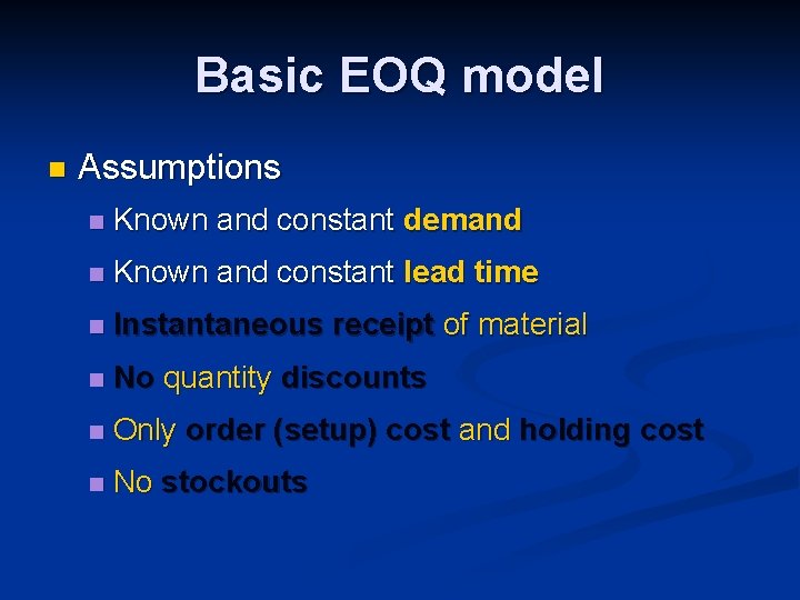
Basic EOQ model n Assumptions n Known and constant demand n Known and constant lead time n Instantaneous receipt of material n No quantity discounts n Only order (setup) cost and holding cost n No stockouts

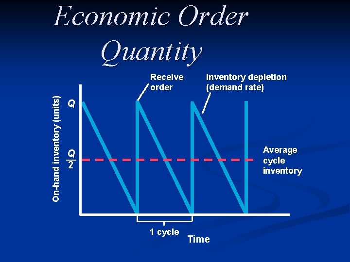
Economic Order Quantity On-hand inventory (units) Receive order Inventory depletion (demand rate) Q Average cycle inventory Q — 2 1 cycle Time

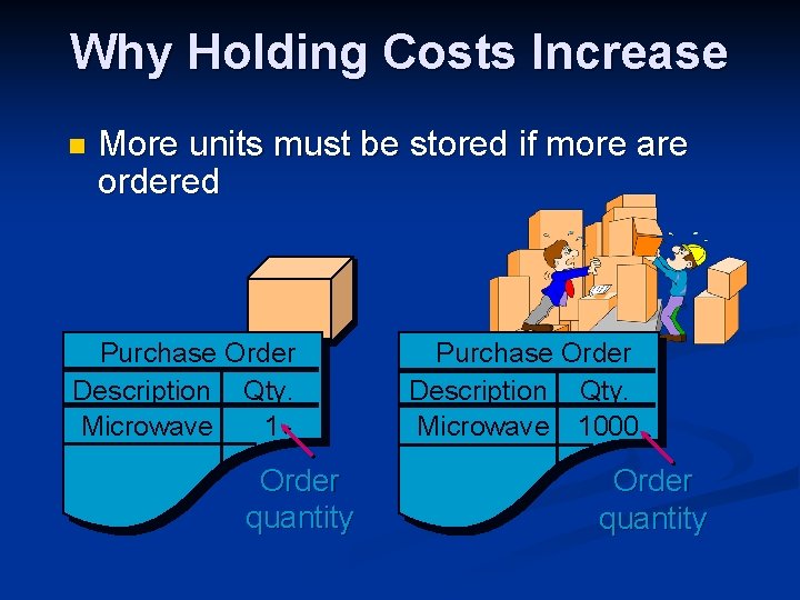
Why Holding Costs Increase n More units must be stored if more are ordered Purchase Order Description Qty. Microwave 1 Order quantity Purchase Order Description Qty. Microwave 1000 Order quantity

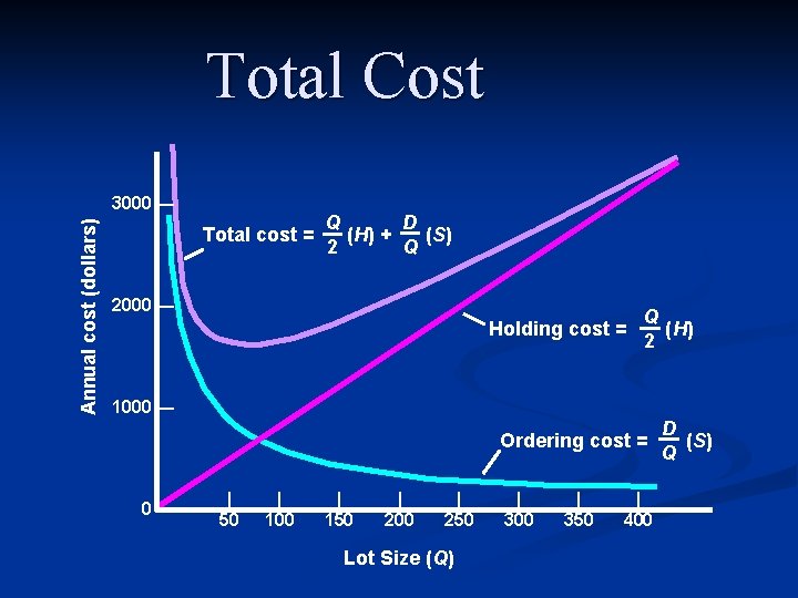
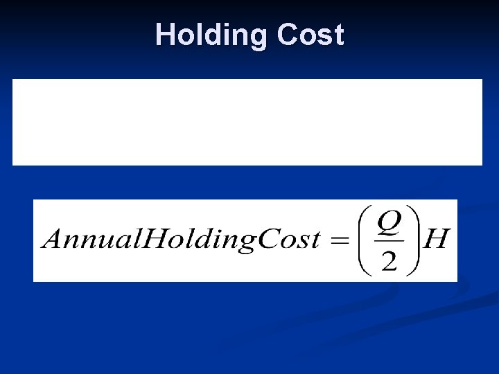
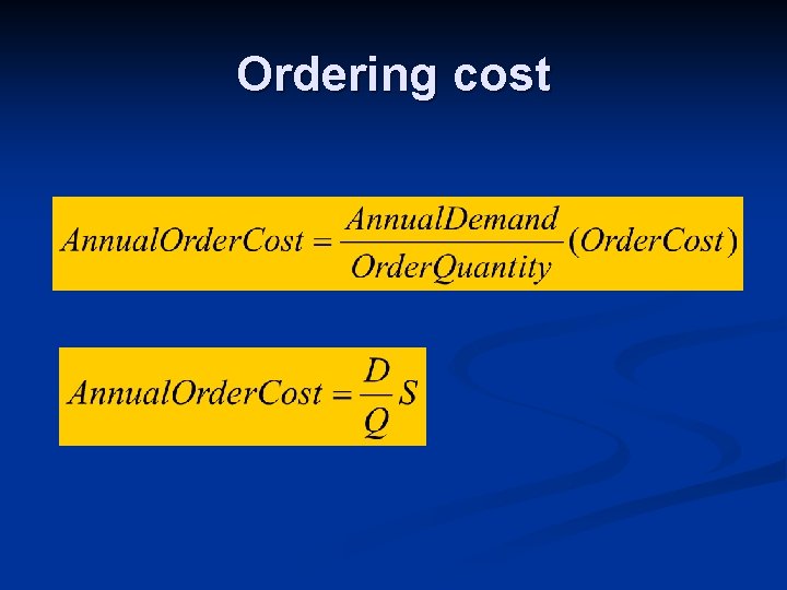
Total Cost Annual cost (dollars) 3000 — Total cost = Q D (H) + (S) 2 Q 2000 — Holding cost = Q (H) 2 1000 — Ordering cost = 0— | 50 | 100 | 150 | 200 | 250 Lot Size (Q) | 300 | 350 | 400 D (S) Q

Holding Cost

Ordering cost

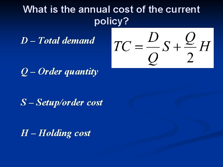
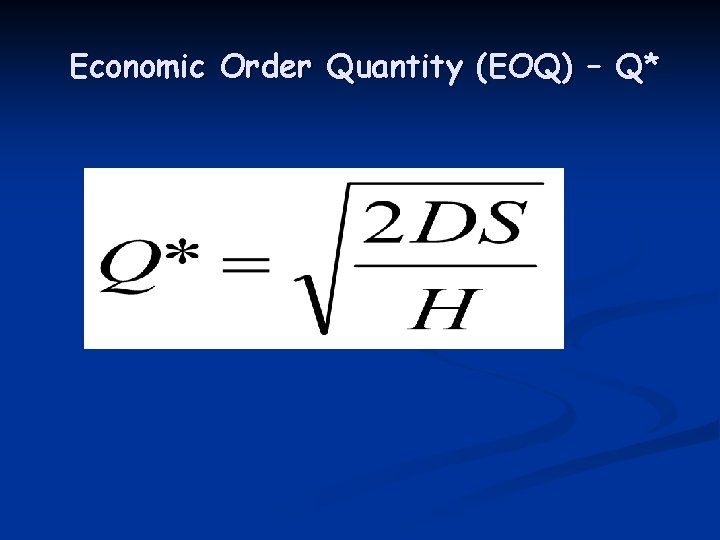
What is the annual cost of the current policy? D – Total demand Q – Order quantity S – Setup/order cost H – Holding cost

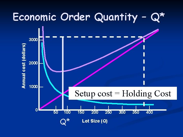
Economic Order Quantity – Q* Annual cost (dollars) 3000 — 2000 — 1000 — 0— Setup cost = Holding Cost | 50 | 100 Q* | 150 | 200 | 250 Lot Size (Q) | 300 | 350 | 400

Economic Order Quantity (EOQ) – Q*

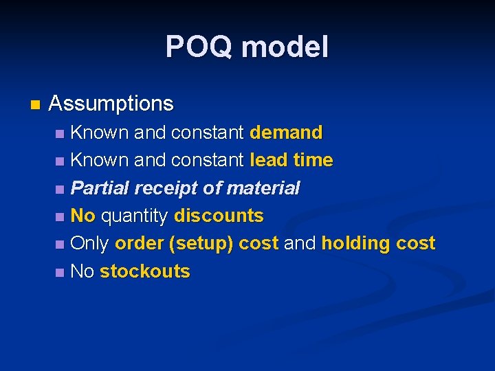
POQ model n Assumptions Known and constant demand n Known and constant lead time n Partial receipt of material n No quantity discounts n Only order (setup) cost and holding cost n No stockouts n

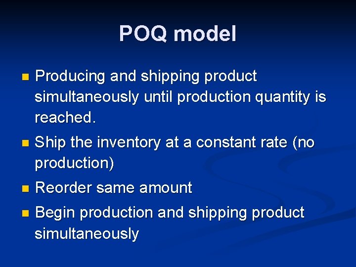
POQ model n Producing and shipping product simultaneously until production quantity is reached. n Ship the inventory at a constant rate (no production) n Reorder same amount n Begin production and shipping product simultaneously

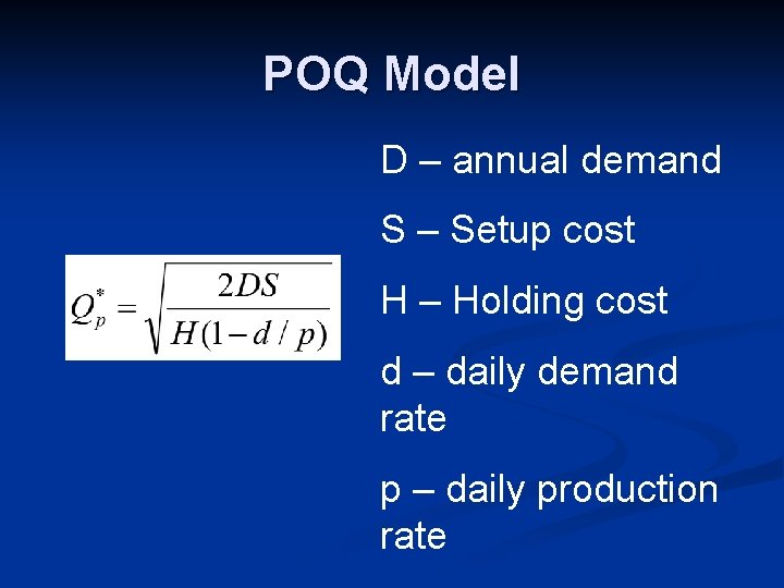
POQ Model D – annual demand S – Setup cost H – Holding cost d – daily demand rate p – daily production rate

Probabilistic Inventory Models n The demand is not known. Demand characteristics such as mean, standard deviation and the distribution of demand may be known. n Stock out cost: The cost associated with a loss of sales when demand cannot be met. 33

Single- and Multi- Period Models n n The classification applies to the probabilistic demand case In a single-period model, the items unsold at the end of the period is not carried over to the next period. The unsold items, however, may have some salvage values. In a multi-period model, all the items unsold at the end of one period are available in the next period. In the single-period model and in some of the multiperiod models, there remains only one question to answer: how much to order. 34

SINGLE-PERIOD MODEL n Computer that will be obsolete before the next order n Perishable product n Seasonal products such as bathing suits, winter coats, etc. n Newspaper and magazine 35

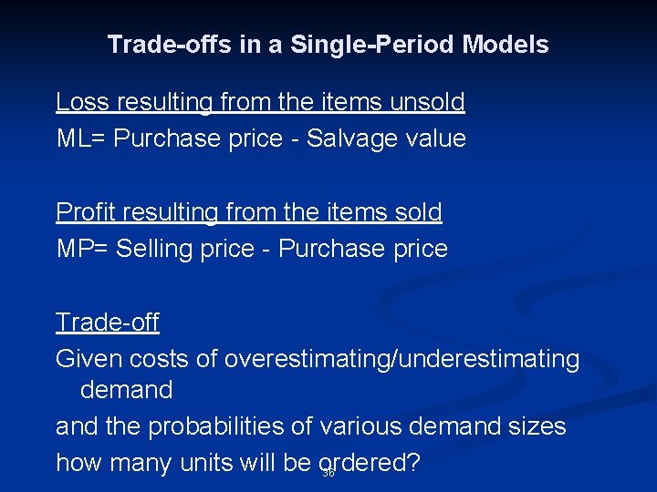
Trade-offs in a Single-Period Models Loss resulting from the items unsold ML= Purchase price - Salvage value Profit resulting from the items sold MP= Selling price - Purchase price Trade-off Given costs of overestimating/underestimating demand the probabilities of various demand sizes how many units will be ordered? 36

MULTI-PERIOD MODELS Outline • A fixed order quantity model • A fixed time period model 37

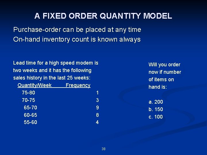
A FIXED ORDER QUANTITY MODEL Purchase-order can be placed at any time On-hand inventory count is known always Lead time for a high speed modem is two weeks and it has the following sales history in the last 25 weeks: Quantity/Week Frequency 75 -80 1 70 -75 3 65 -70 9 60 -65 8 55 -60 4 Will you order now if number of items on hand is: a. 200 b. 150 c. 100 38

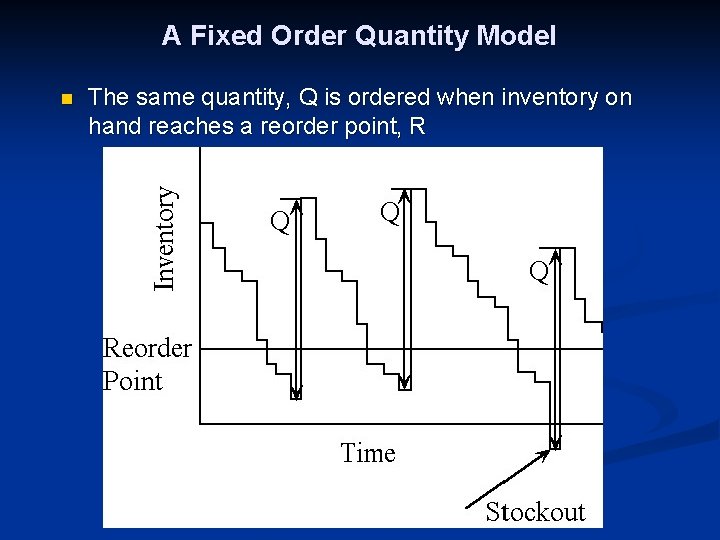
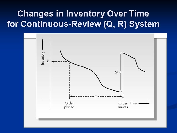
A Fixed Order Quantity Model n The same quantity, Q is ordered when inventory on hand reaches a reorder point, R 39

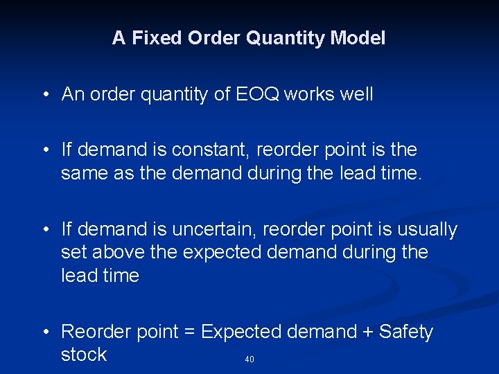
A Fixed Order Quantity Model • An order quantity of EOQ works well • If demand is constant, reorder point is the same as the demand during the lead time. • If demand is uncertain, reorder point is usually set above the expected demand during the lead time • Reorder point = Expected demand + Safety stock 40

A FIXED TIME PERIOD MODEL • Purchase-order is issued at a fixed interval of time A distributor of soft drinks prepares a purchase order for beverages once a week on every Monday. The beverages are received on Thursdays (the lead time is three days). Choose a method for finding order quantity for the distributor: a. Mean demand for 7 days + safety stock b. Mean demand for 10 days + safety stock c. Mean demand for 10 days + safety stock — inventory on hand 41

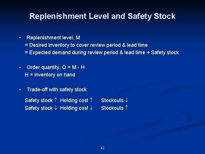
Replenishment Level and Safety Stock • Replenishment level, M = Desired inventory to cover review period & lead time = Expected demand during review period & lead time + Safety stock • Order quantity, Q = M - H H = inventory on hand • Trade-off with safety stock Safety stock Holding cost Stockouts 42

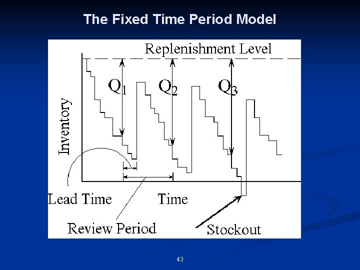
The Fixed Time Period Model 43

Decision Variables n n For the basic EOQ model discussed in Chapter 4, there was only the single decision variable Q. The value of the reorder level, R, was determined by Q. Now we treat Q and R as independent decision variables. Essentially, R is chosen to protect against uncertainty of demand during the lead time, and Q is chosen to balance the holding and set-up costs. (Refer to Figure 5 -5)

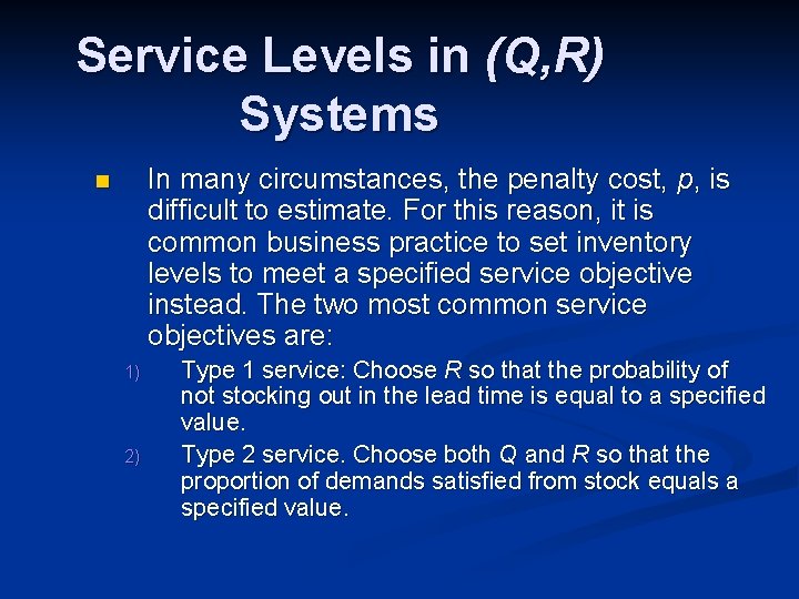
Service Levels in (Q, R) Systems In many circumstances, the penalty cost, p, is difficult to estimate. For this reason, it is common business practice to set inventory levels to meet a specified service objective instead. The two most common service objectives are: n 1) 2) Type 1 service: Choose R so that the probability of not stocking out in the lead time is equal to a specified value. Type 2 service. Choose both Q and R so that the proportion of demands satisfied from stock equals a specified value.

Changes in Inventory Over Time for Continuous-Review (Q, R) System

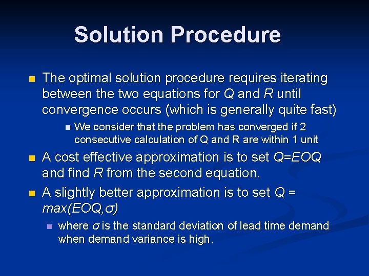
Solution Procedure n The optimal solution procedure requires iterating between the two equations for Q and R until convergence occurs (which is generally quite fast) n n n We consider that the problem has converged if 2 consecutive calculation of Q and R are within 1 unit A cost effective approximation is to set Q=EOQ and find R from the second equation. A slightly better approximation is to set Q = max(EOQ, σ) n where σ is the standard deviation of lead time demand when demand variance is high.

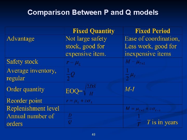
Comparison Between P and Q models 48

When to order? n Reorder point (ROP) n Lead time – amount of time from order placement to receipt of goods n Lead time demand – the demand the occurs during the lead time

THANK YOU