Inventory Management 12 Power Point presentation to accompany

Inventory Management 12 Power. Point presentation to accompany Heizer and Render Operations Management, Eleventh Edition Principles of Operations Management, Ninth Edition Power. Point slides by Jeff Heyl © 2014 Pearson Education, Inc. 12 - 1

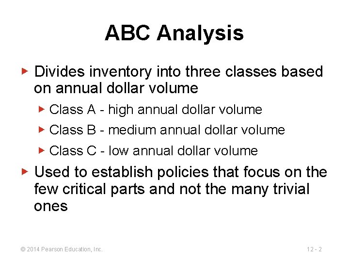
ABC Analysis ▶ Divides inventory into three classes based on annual dollar volume ▶ Class A - high annual dollar volume ▶ Class B - medium annual dollar volume ▶ Class C - low annual dollar volume ▶ Used to establish policies that focus on the few critical parts and not the many trivial ones © 2014 Pearson Education, Inc. 12 - 2

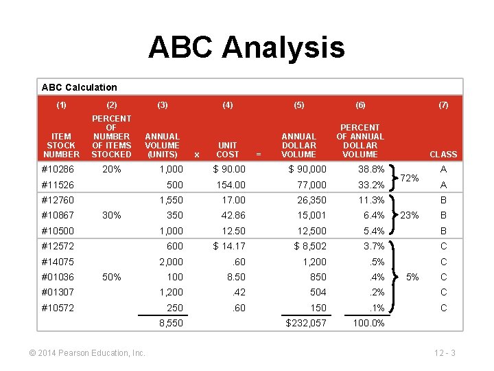
ABC Analysis ABC Calculation (1) (2) (3) ITEM STOCK NUMBER PERCENT OF NUMBER OF ITEMS STOCKED ANNUAL VOLUME (UNITS) #10286 (5) (6) (7) UNIT COST ANNUAL DOLLAR VOLUME PERCENT OF ANNUAL DOLLAR VOLUME CLASS = 1, 000 $ 90, 000 38. 8% #11526 500 154. 00 77, 000 33. 2% #12760 1, 550 17. 00 26, 350 11. 3% 350 42. 86 15, 001 6. 4% #10500 1, 000 12. 50 12, 500 5. 4% B #12572 600 $ 14. 17 $ 8, 502 3. 7% C #14075 2, 000 . 60 1, 200 . 5% C 100 8. 50 850 . 4% #01307 1, 200 . 42 504 . 2% C #10572 250 . 60 150 . 1% C $232, 057 100. 0% #10867 #01036 20% x (4) 30% 50% 8, 550 © 2014 Pearson Education, Inc. 72% A A B 23% 5% B C 12 - 3

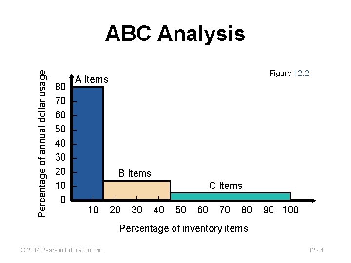
Percentage of annual dollar usage ABC Analysis 80 70 60 50 40 30 20 10 0 A Items – – – – B Items – | | – 10 20 30 40 Figure 12. 2 C Items | | 50 60 70 80 | | 90 100 Percentage of inventory items © 2014 Pearson Education, Inc. 12 - 4

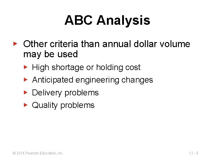
ABC Analysis ▶ Other criteria than annual dollar volume may be used ▶ ▶ High shortage or holding cost Anticipated engineering changes Delivery problems Quality problems © 2014 Pearson Education, Inc. 12 - 5

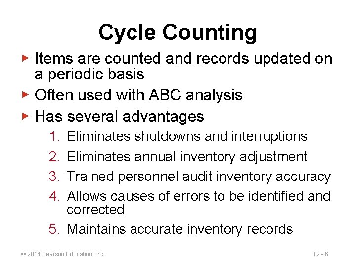
Cycle Counting ▶ Items are counted and records updated on a periodic basis ▶ Often used with ABC analysis ▶ Has several advantages 1. 2. 3. 4. Eliminates shutdowns and interruptions Eliminates annual inventory adjustment Trained personnel audit inventory accuracy Allows causes of errors to be identified and corrected 5. Maintains accurate inventory records © 2014 Pearson Education, Inc. 12 - 6

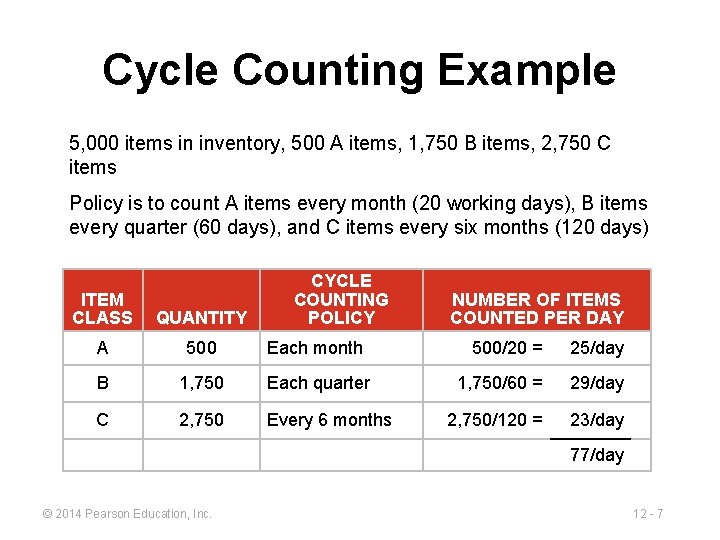
Cycle Counting Example 5, 000 items in inventory, 500 A items, 1, 750 B items, 2, 750 C items Policy is to count A items every month (20 working days), B items every quarter (60 days), and C items every six months (120 days) CYCLE COUNTING POLICY ITEM CLASS QUANTITY A 500 Each month B 1, 750 Each quarter C 2, 750 Every 6 months NUMBER OF ITEMS COUNTED PER DAY 500/20 = 25/day 1, 750/60 = 29/day 2, 750/120 = 23/day 77/day © 2014 Pearson Education, Inc. 12 - 7

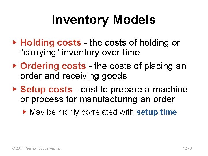
Inventory Models ▶ Holding costs - the costs of holding or “carrying” inventory over time ▶ Ordering costs - the costs of placing an order and receiving goods ▶ Setup costs - cost to prepare a machine or process for manufacturing an order ▶ May be highly correlated with setup time © 2014 Pearson Education, Inc. 12 - 8

Inventory Models for Independent Demand Need to determine when and how much to order 1. Basic economic order quantity (EOQ) model 2. Production order quantity model 3. Quantity discount model © 2014 Pearson Education, Inc. 12 - 9

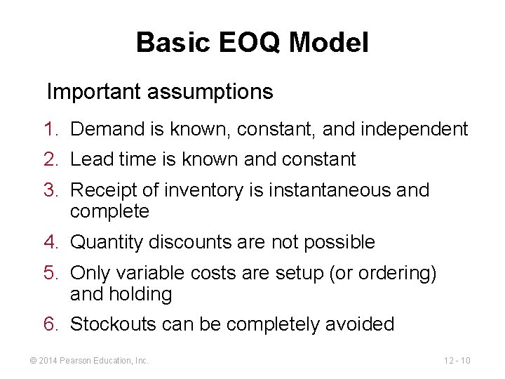
Basic EOQ Model Important assumptions 1. Demand is known, constant, and independent 2. Lead time is known and constant 3. Receipt of inventory is instantaneous and complete 4. Quantity discounts are not possible 5. Only variable costs are setup (or ordering) and holding 6. Stockouts can be completely avoided © 2014 Pearson Education, Inc. 12 - 10

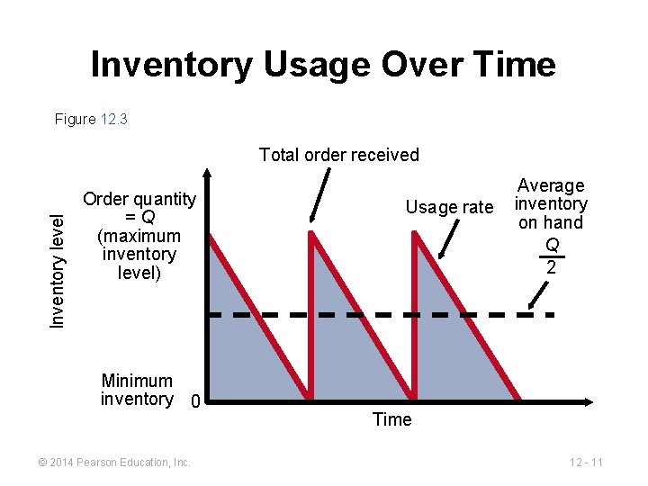
Inventory Usage Over Time Figure 12. 3 Inventory level Total order received Order quantity =Q (maximum inventory level) Minimum inventory 0 © 2014 Pearson Education, Inc. Usage rate Average inventory on hand Q 2 Time 12 - 11

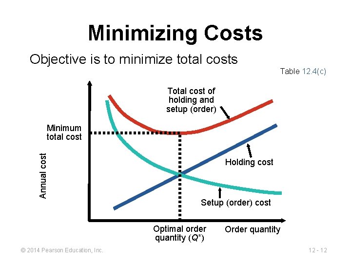
Minimizing Costs Objective is to minimize total costs Table 12. 4(c) Total cost of holding and setup (order) Annual cost Minimum total cost Holding cost Setup (order) cost Optimal order quantity (Q*) © 2014 Pearson Education, Inc. Order quantity 12 - 12

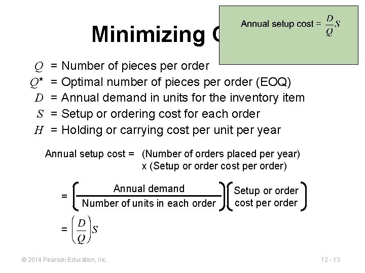
Minimizing Costs Q Q* D S H = Number of pieces per order = Optimal number of pieces per order (EOQ) = Annual demand in units for the inventory item = Setup or ordering cost for each order = Holding or carrying cost per unit per year Annual setup cost = (Number of orders placed per year) x (Setup or order cost per order) = Annual demand Number of units in each order © 2014 Pearson Education, Inc. Setup or order cost per order 12 - 13

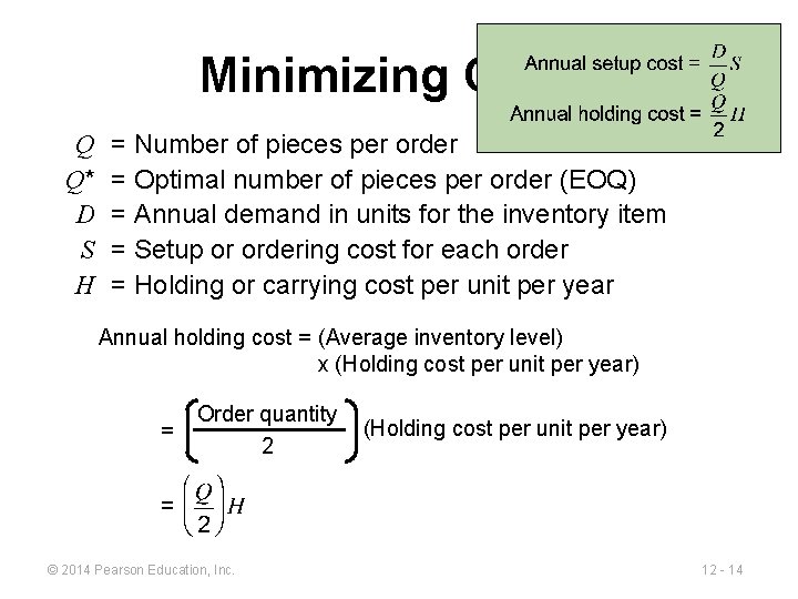
Minimizing Costs Q Q* D S H = Number of pieces per order = Optimal number of pieces per order (EOQ) = Annual demand in units for the inventory item = Setup or ordering cost for each order = Holding or carrying cost per unit per year Annual holding cost = (Average inventory level) x (Holding cost per unit per year) = Order quantity 2 © 2014 Pearson Education, Inc. (Holding cost per unit per year) 12 - 14

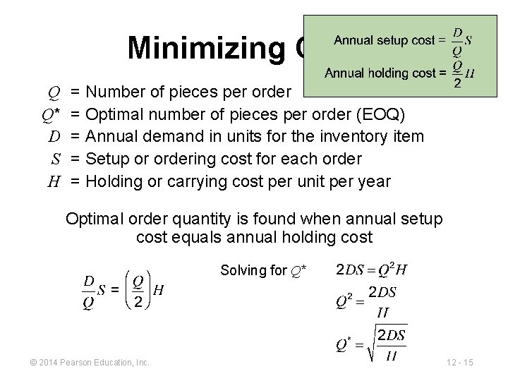
Minimizing Costs Q Q* D S H = Number of pieces per order = Optimal number of pieces per order (EOQ) = Annual demand in units for the inventory item = Setup or ordering cost for each order = Holding or carrying cost per unit per year Optimal order quantity is found when annual setup cost equals annual holding cost Solving for Q* © 2014 Pearson Education, Inc. 12 - 15

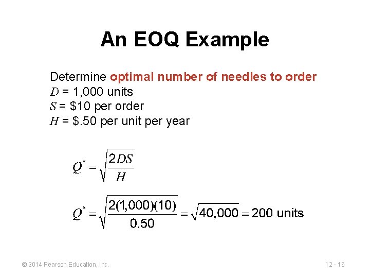
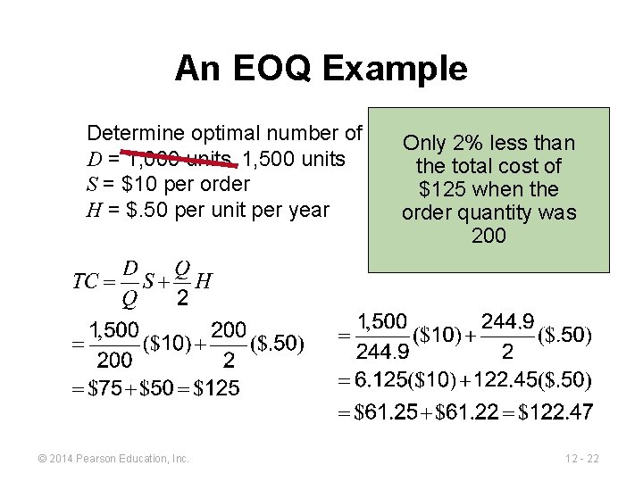
An EOQ Example Determine optimal number of needles to order D = 1, 000 units S = $10 per order H = $. 50 per unit per year © 2014 Pearson Education, Inc. 12 - 16

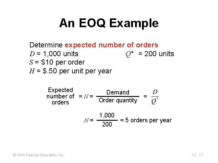
An EOQ Example Determine expected number of orders D = 1, 000 units Q* = 200 units S = $10 per order H = $. 50 per unit per year Expected Demand number of = N = Order quantity orders = 1, 000 N= = 5 orders per year 200 © 2014 Pearson Education, Inc. 12 - 17

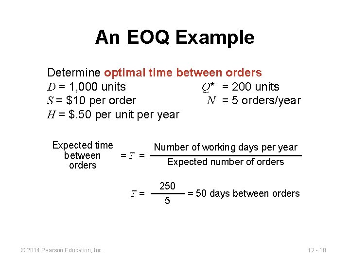
An EOQ Example Determine optimal time between orders D = 1, 000 units Q* = 200 units S = $10 per order N = 5 orders/year H = $. 50 per unit per year Expected time Number of working days per year between =T = Expected number of orders T= © 2014 Pearson Education, Inc. 250 5 = 50 days between orders 12 - 18

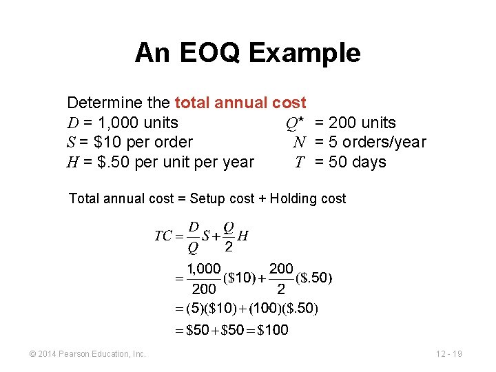
An EOQ Example Determine the total annual cost D = 1, 000 units Q* = 200 units S = $10 per order N = 5 orders/year H = $. 50 per unit per year T = 50 days Total annual cost = Setup cost + Holding cost © 2014 Pearson Education, Inc. 12 - 19

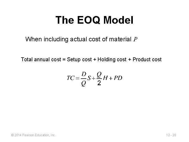
The EOQ Model When including actual cost of material P Total annual cost = Setup cost + Holding cost + Product cost © 2014 Pearson Education, Inc. 12 - 20

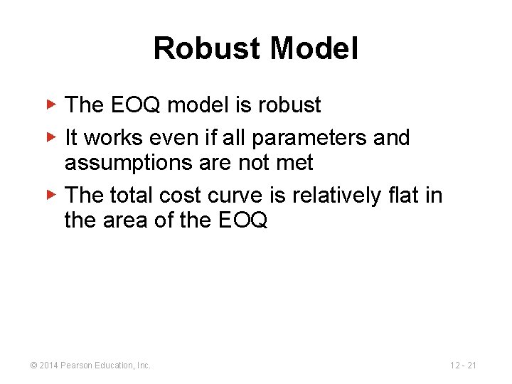
Robust Model ▶ The EOQ model is robust ▶ It works even if all parameters and assumptions are not met ▶ The total cost curve is relatively flat in the area of the EOQ © 2014 Pearson Education, Inc. 12 - 21

An EOQ Example Determine optimal number of needles Only to 2%order less than D = 1, 000 units 1, 500 units Q* =the 200 total units cost of S = $10 per order N =$125 5 orders/year when the H = $. 50 per unit per year T order = 50 days quantity was 200 © 2014 Pearson Education, Inc. 12 - 22

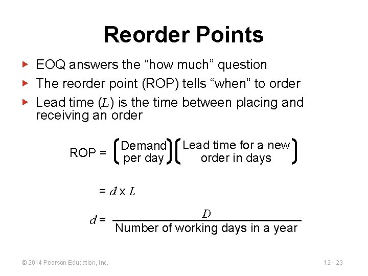
Reorder Points ▶ EOQ answers the “how much” question ▶ The reorder point (ROP) tells “when” to order ▶ Lead time (L) is the time between placing and receiving an order ROP = Demand per day Lead time for a new order in days =dx. L d= © 2014 Pearson Education, Inc. D Number of working days in a year 12 - 23

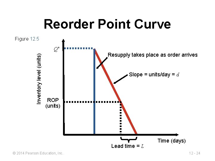
Reorder Point Curve Figure 12. 5 Inventory level (units) Q* Resupply takes place as order arrives Slope = units/day = d ROP (units) Lead time = L © 2014 Pearson Education, Inc. Time (days) 12 - 24

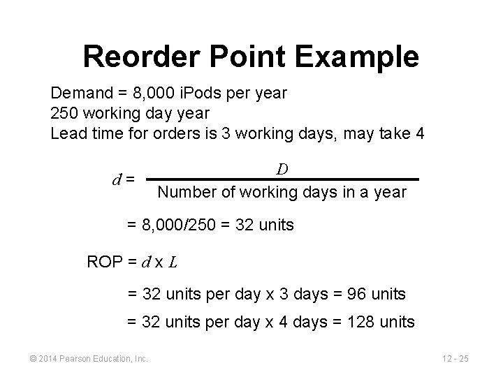
Reorder Point Example Demand = 8, 000 i. Pods per year 250 working day year Lead time for orders is 3 working days, may take 4 d= D Number of working days in a year = 8, 000/250 = 32 units ROP = d x L = 32 units per day x 3 days = 96 units = 32 units per day x 4 days = 128 units © 2014 Pearson Education, Inc. 12 - 25

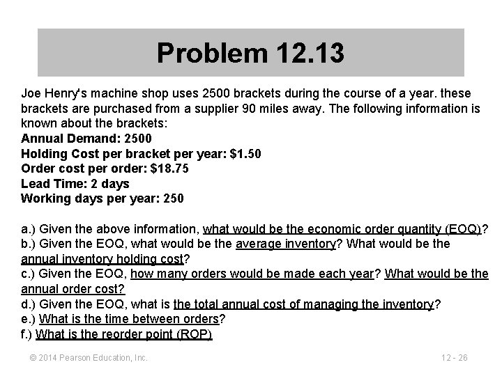
Problem 12. 13 Joe Henry's machine shop uses 2500 brackets during the course of a year. these brackets are purchased from a supplier 90 miles away. The following information is known about the brackets: Annual Demand: 2500 Holding Cost per bracket per year: $1. 50 Order cost per order: $18. 75 Lead Time: 2 days Working days per year: 250 a. ) Given the above information, what would be the economic order quantity (EOQ)? b. ) Given the EOQ, what would be the average inventory? What would be the annual inventory holding cost? c. ) Given the EOQ, how many orders would be made each year? What would be the annual order cost? d. ) Given the EOQ, what is the total annual cost of managing the inventory? e. ) What is the time between orders? f. ) What is the reorder point (ROP) © 2014 Pearson Education, Inc. 12 - 26

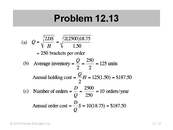
Problem 12. 13 © 2014 Pearson Education, Inc. 12 - 27

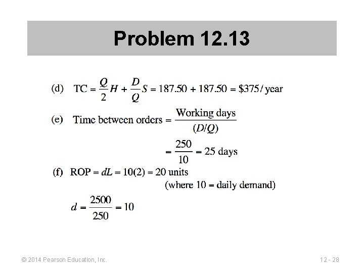
Problem 12. 13 © 2014 Pearson Education, Inc. 12 - 28

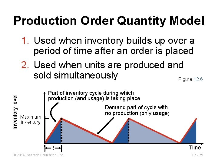
Production Order Quantity Model Inventory level 1. Used when inventory builds up over a period of time after an order is placed 2. Used when units are produced and sold simultaneously Figure 12. 6 Part of inventory cycle during which production (and usage) is taking place Demand part of cycle with no production (only usage) Maximum inventory t © 2014 Pearson Education, Inc. Time 12 - 29

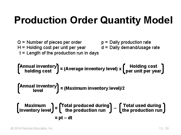
Production Order Quantity Model Q = Number of pieces per order p = Daily production rate H = Holding cost per unit per year d = Daily demand/usage rate t = Length of the production run in days Holding cost Annual inventory = (Average inventory level) x per unit per year holding cost Annual inventory = (Maximum inventory level)/2 level Maximum Total produced during = – inventory level the production run Total used during the production run = pt – dt © 2014 Pearson Education, Inc. 12 - 30

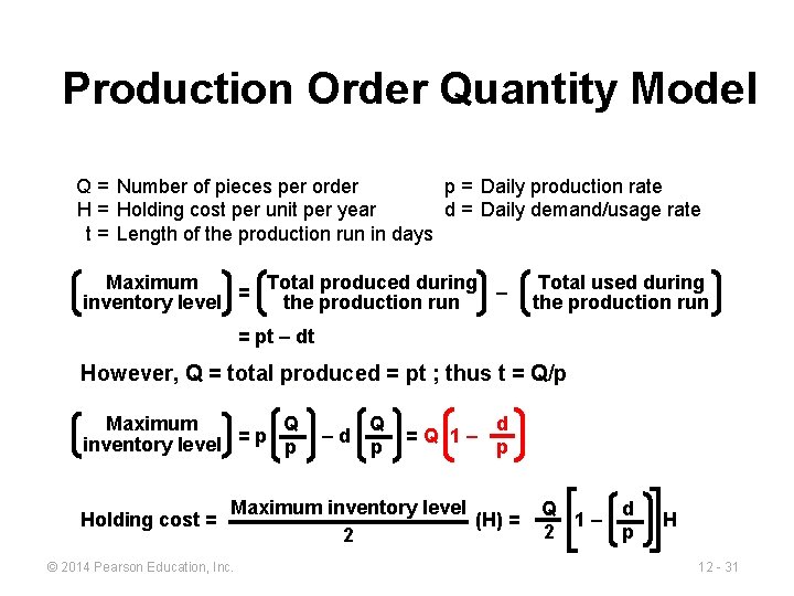
Production Order Quantity Model Q = Number of pieces per order p = Daily production rate H = Holding cost per unit per year d = Daily demand/usage rate t = Length of the production run in days Maximum Total produced during = – inventory level the production run Total used during the production run = pt – dt However, Q = total produced = pt ; thus t = Q/p Q Maximum = p inventory level p Holding cost = –d Q p =Q 1– d p Maximum inventory level (H) = 2 © 2014 Pearson Education, Inc. d Q 1– p 2 H 12 - 31

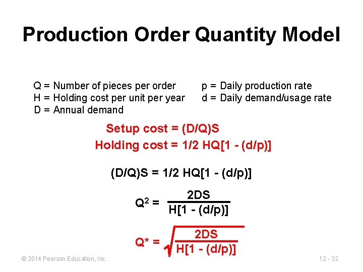
Production Order Quantity Model Q = Number of pieces per order H = Holding cost per unit per year D = Annual demand p = Daily production rate d = Daily demand/usage rate Setup cost = (D/Q)S Holding cost = 1/2 HQ[1 - (d/p)] (D/Q)S = 1/2 HQ[1 - (d/p)] Q 2 2 DS = H[1 - (d/p)] Q* = © 2014 Pearson Education, Inc. 2 DS H[1 - (d/p)] 12 - 32

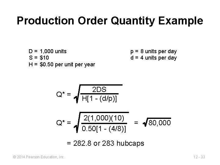
Production Order Quantity Example D= S= H= 1, 000 units $10 $0. 50 per unit per year Q* = 2 DS H[1 - (d/p)] Q* = 2(1, 000)(10) 0. 50[1 - (4/8)] p = 8 units per day d = 4 units per day = 80, 000 = 282. 8 or 283 hubcaps © 2014 Pearson Education, Inc. 12 - 33

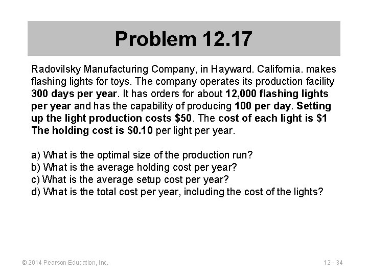
Problem 12. 17 Radovilsky Manufacturing Company, in Hayward. California. makes flashing lights for toys. The company operates its production facility 300 days per year. It has orders for about 12, 000 flashing lights per year and has the capability of producing 100 per day. Setting up the light production costs $50. The cost of each light is $1 The holding cost is $0. 10 per light per year. a) What is the optimal size of the production run? b) What is the average holding cost per year? c) What is the average setup cost per year? d) What is the total cost per year, including the cost of the lights? © 2014 Pearson Education, Inc. 12 - 34

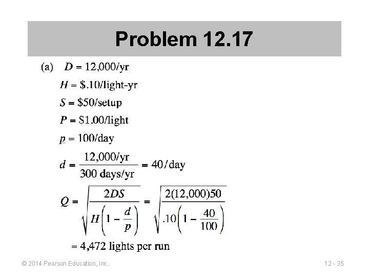
Problem 12. 17 © 2014 Pearson Education, Inc. 12 - 35

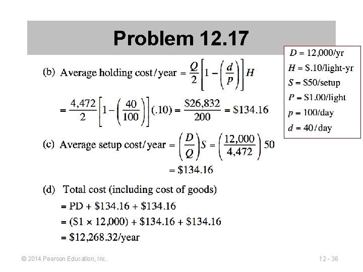
Problem 12. 17 © 2014 Pearson Education, Inc. 12 - 36

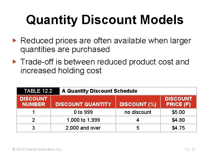
Quantity Discount Models ▶ Reduced prices are often available when larger quantities are purchased ▶ Trade-off is between reduced product cost and increased holding cost TABLE 12. 2 A Quantity Discount Schedule DISCOUNT NUMBER DISCOUNT QUANTITY DISCOUNT (%) 1 0 to 999 no discount 2 1, 000 to 1, 999 4 3 © 2014 Pearson Education, Inc. 2, 000 and over 5 DISCOUNT PRICE (P) $5. 00 $4. 80 $4. 75 12 - 37

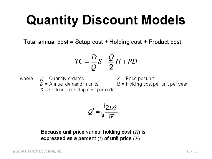
Quantity Discount Models Total annual cost = Setup cost + Holding cost + Product cost where Q = Quantity ordered P = Price per unit D = Annual demand in units H = Holding cost per unit per year S = Ordering or setup cost per order Because unit price varies, holding cost (H) is expressed as a percent (I) of unit price (P) © 2014 Pearson Education, Inc. 12 - 38

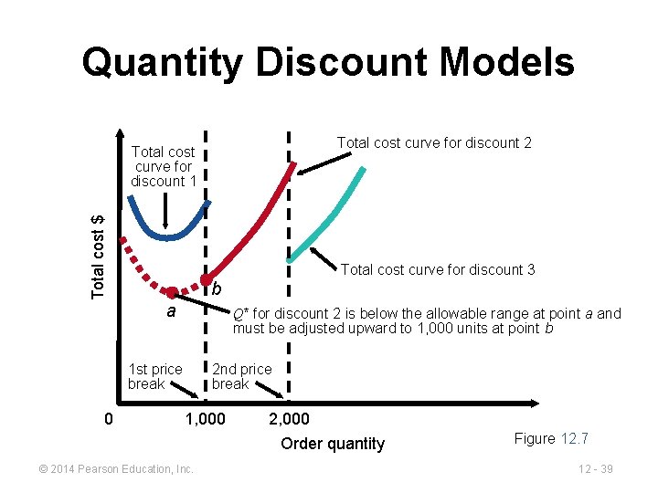
Quantity Discount Models Total cost curve for discount 2 Total cost $ Total cost curve for discount 1 Total cost curve for discount 3 b a Q* for discount 2 is below the allowable range at point a and must be adjusted upward to 1, 000 units at point b 1 st price break 0 2 nd price break 1, 000 2, 000 Order quantity © 2014 Pearson Education, Inc. Figure 12. 7 12 - 39

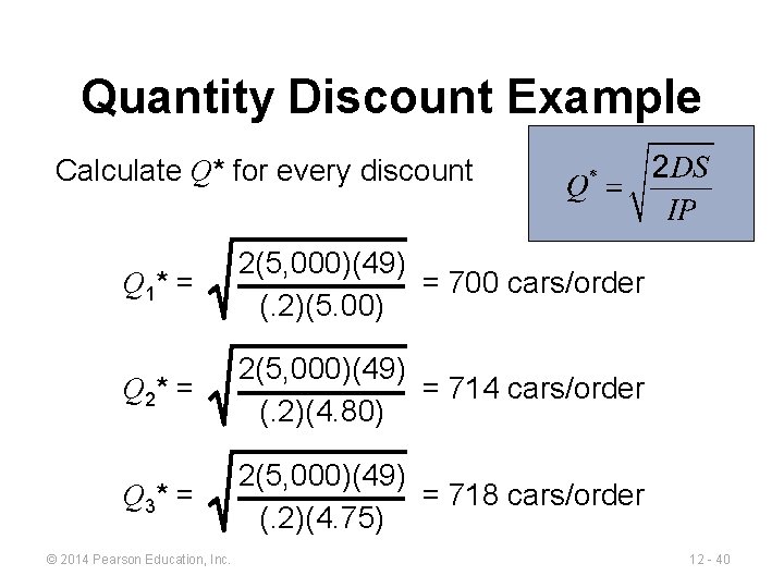
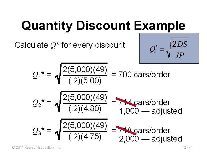
Quantity Discount Example Calculate Q* for every discount Q 1* = 2(5, 000)(49) = 700 cars/order (. 2)(5. 00) Q 2* = 2(5, 000)(49) = 714 cars/order (. 2)(4. 80) Q 3* = 2(5, 000)(49) = 718 cars/order (. 2)(4. 75) © 2014 Pearson Education, Inc. 12 - 40

Quantity Discount Example Calculate Q* for every discount Q 1* = 2(5, 000)(49) = 700 cars/order (. 2)(5. 00) Q 2* = 2(5, 000)(49) = 714 cars/order (. 2)(4. 80) 1, 000 — adjusted Q 3* = 2(5, 000)(49) = 718 cars/order (. 2)(4. 75) 2, 000 — adjusted © 2014 Pearson Education, Inc. 12 - 41

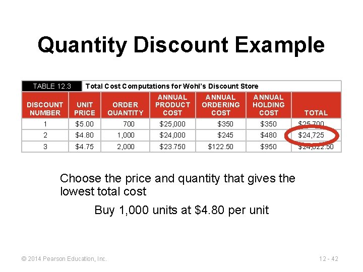
Quantity Discount Example TABLE 12. 3 Total Cost Computations for Wohl’s Discount Store ORDER QUANTITY ANNUAL PRODUCT COST ANNUAL ORDERING COST ANNUAL HOLDING COST DISCOUNT NUMBER UNIT PRICE 1 $5. 00 700 $25, 000 $350 $25, 700 2 $4. 80 1, 000 $245 $480 $24, 725 3 $4. 75 2, 000 $23. 750 $122. 50 $950 $24, 822. 50 TOTAL Choose the price and quantity that gives the lowest total cost Buy 1, 000 units at $4. 80 per unit © 2014 Pearson Education, Inc. 12 - 42

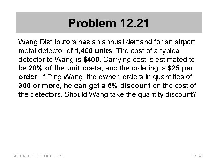
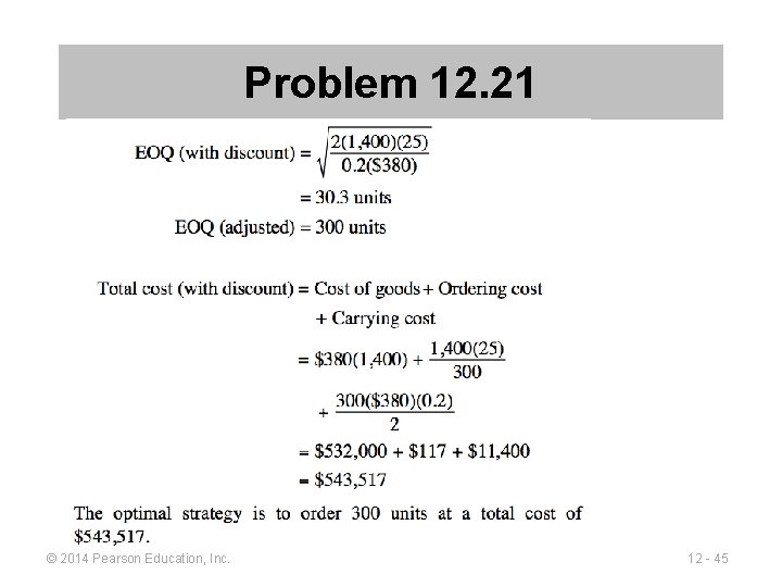
Problem 12. 21 Wang Distributors has an annual demand for an airport metal detector of 1, 400 units. The cost of a typical detector to Wang is $400. Carrying cost is estimated to be 20% of the unit costs, and the ordering is $25 per order. If Ping Wang, the owner, orders in quantities of 300 or more, he can get a 5% discount on the cost of the detectors. Should Wang take the quantity discount? © 2014 Pearson Education, Inc. 12 - 43

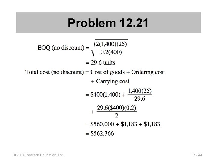
Problem 12. 21 © 2014 Pearson Education, Inc. 12 - 44

Problem 12. 21 © 2014 Pearson Education, Inc. 12 - 45