Introduction to the Mathematics of Image and Data

Introduction to the Mathematics of Image and Data Analysis Math 5467, Spring 2015 Instructor: Gilad Lerman lerman@umn. edu

What’s the course is about? • Mathematical techniques (Fourier, wavelets, SVD, etc. ) • Problems from data analysis (mainly image analysis)

Digital Images and Problems

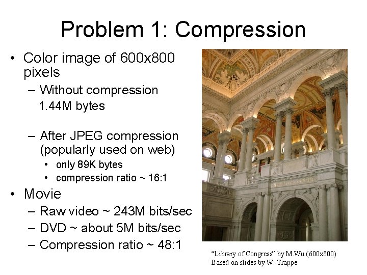
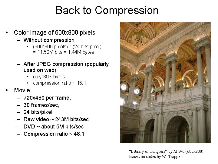
Problem 1: Compression • Color image of 600 x 800 pixels – Without compression 1. 44 M bytes – After JPEG compression (popularly used on web) • only 89 K bytes • compression ratio ~ 16: 1 • Movie – Raw video ~ 243 M bits/sec – DVD ~ about 5 M bits/sec – Compression ratio ~ 48: 1 “Library of Congress” by M. Wu (600 x 800) Based on slides by W. Trappe

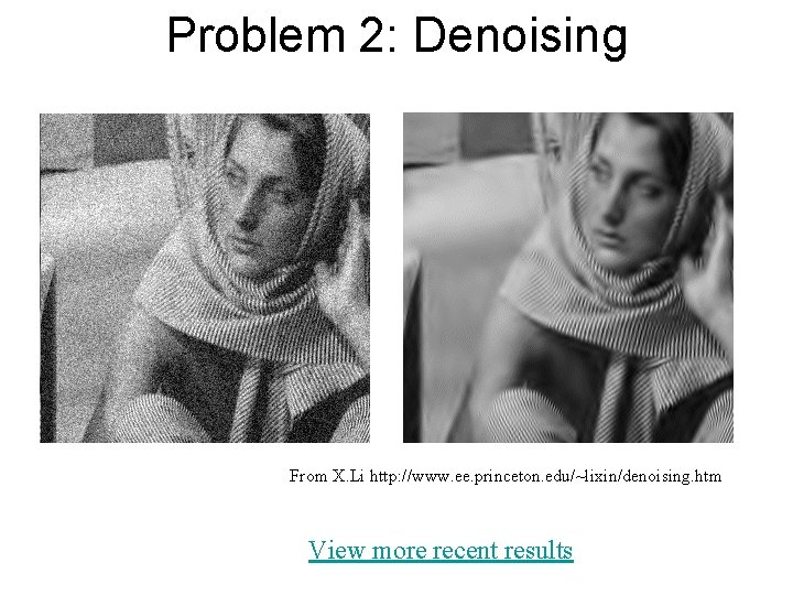
Problem 2: Denoising From X. Li http: //www. ee. princeton. edu/~lixin/denoising. htm View more recent results

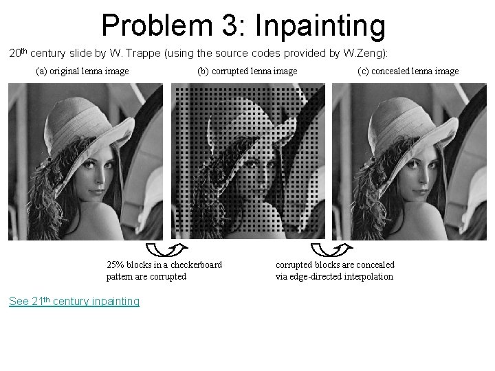
Problem 3: Inpainting 20 th century slide by W. Trappe (using the source codes provided by W. Zeng): (a) original lenna image (b) corrupted lenna image 25% blocks in a checkerboard pattern are corrupted See 21 th century inpainting (c) concealed lenna image corrupted blocks are concealed via edge-directed interpolation

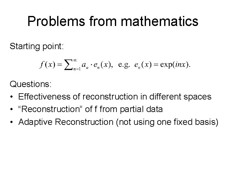
Problems from mathematics Starting point: Questions: • Effectiveness of reconstruction in different spaces • “Reconstruction” of f from partial data • Adaptive Reconstruction (not using one fixed basis)

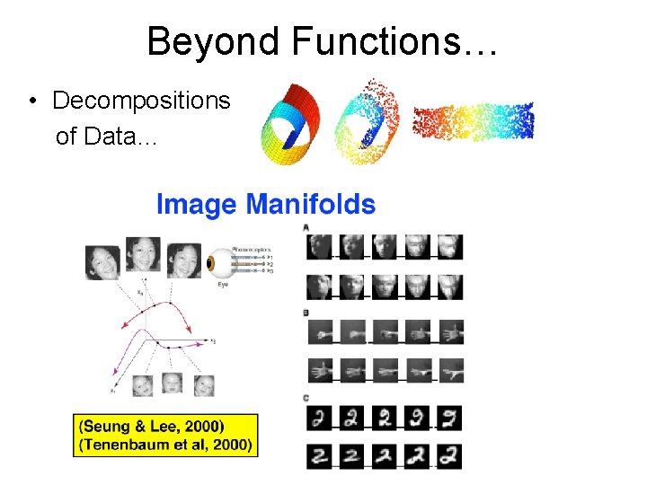
Beyond Functions… • Decompositions of Data…

Class plan • Quick introduction to images • Singular value decomposition (adaptive representation) • Hilbert spaces and normed spaces • Basic Fourier analysis and image analysis in the frequency domain • Convolution and low/high pass spatial filters • Image restoration • Wavelet analysis • Image compression (if time allows) • Sparse approximation and compressed sensing (if time allows)

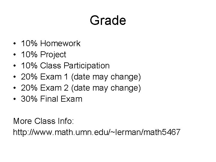
Grade • • • 10% Homework 10% Project 10% Class Participation 20% Exam 1 (date may change) 20% Exam 2 (date may change) 30% Final Exam More Class Info: http: //www. math. umn. edu/~lerman/math 5467

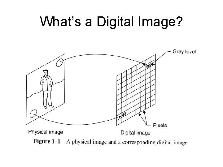
What’s a Digital Image?

Mechanism for digitizing

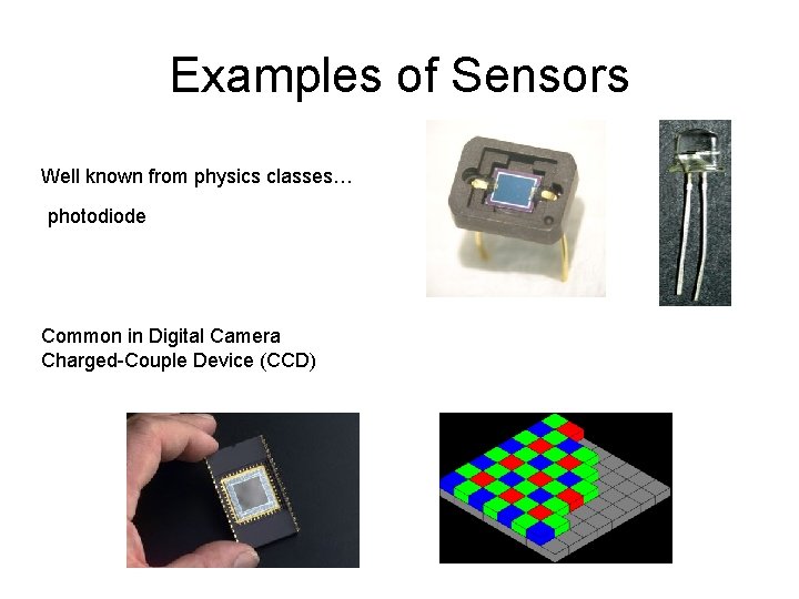
Examples of Sensors Well known from physics classes… photodiode Common in Digital Camera Charged-Couple Device (CCD)

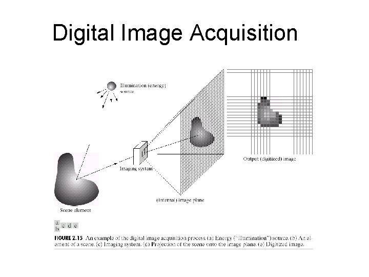
Digital Image Acquisition

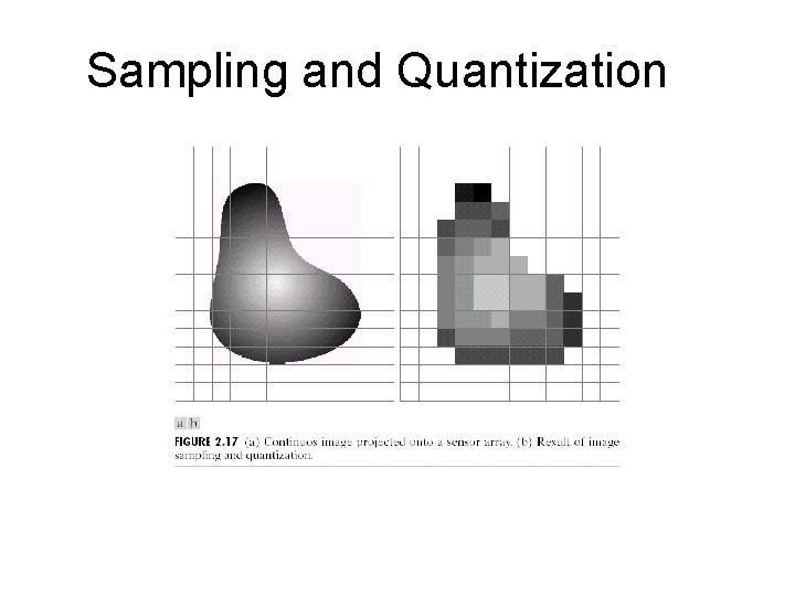
Sampling and Quantization

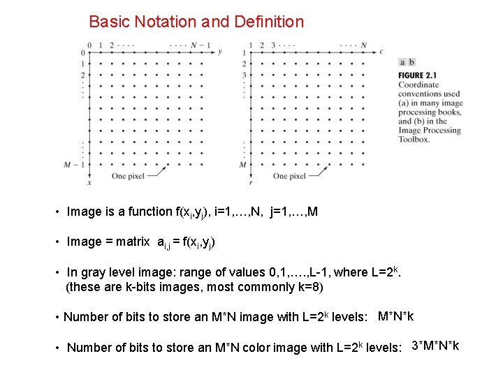
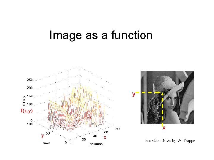
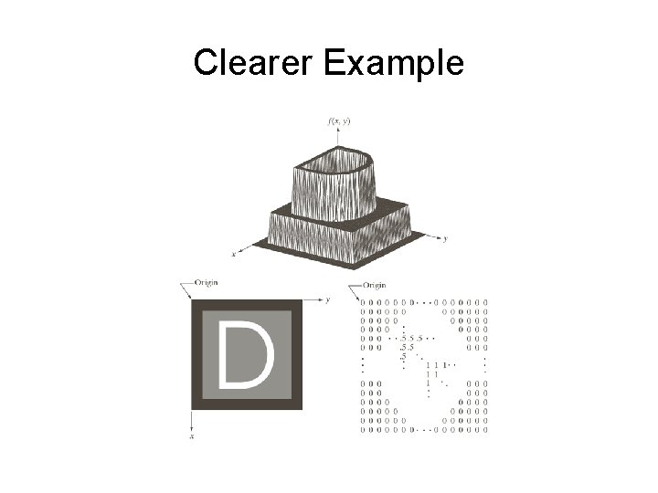
Basic Notation and Definition • Image is a function f(xi, yj), i=1, …, N, j=1, …, M • Image = matrix ai, j = f(xi, yj) • In gray level image: range of values 0, 1, …. , L-1, where L=2 k. (these are k-bits images, most commonly k=8) • Number of bits to store an M*N image with L=2 k levels: M*N*k • Number of bits to store an M*N color image with L=2 k levels: 3*M*N*k

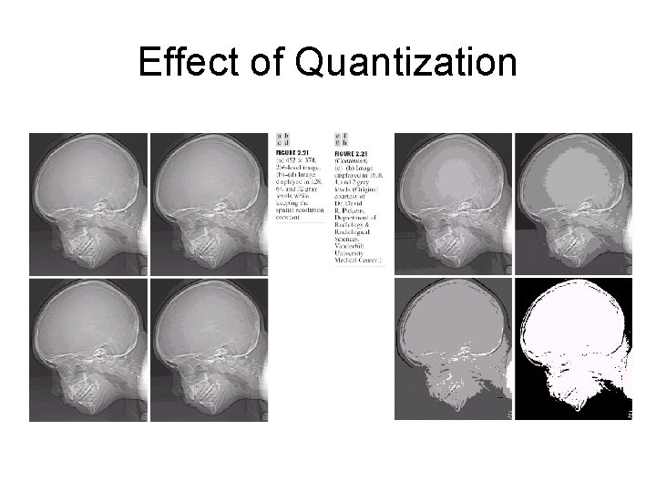
Effect of Quantization

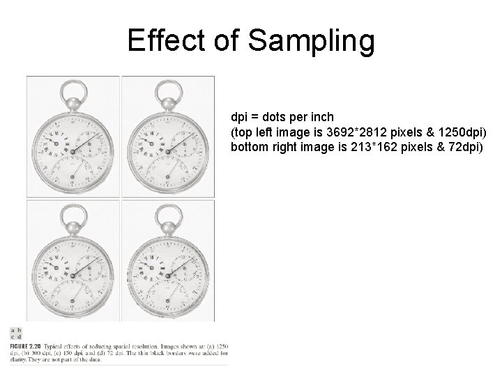
Effect of Sampling dpi = dots per inch (top left image is 3692*2812 pixels & 1250 dpi) bottom right image is 213*162 pixels & 72 dpi)

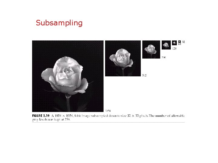
Subsampling

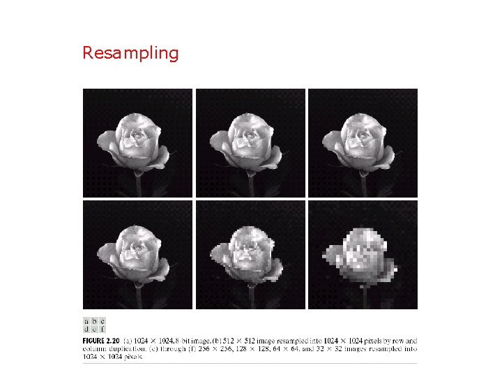
Resampling

Back to Compression • Color image of 600 x 800 pixels – Without compression • (600*800 pixels) * (24 bits/pixel) = 11. 52 M bits = 1. 44 M bytes – After JPEG compression (popularly used on web) • • only 89 K bytes compression ratio ~ 16: 1 • Movie – – – 720 x 480 per frame, 30 frames/sec, 24 bits/pixel Raw video ~ 243 M bits/sec DVD ~ about 5 M bits/sec Compression ratio ~ 48: 1 “Library of Congress” by M. Wu (600 x 800) Based on slides by W. Trappe

Image as a function y I(x, y) x y x Based on slides by W. Trappe

Clearer Example

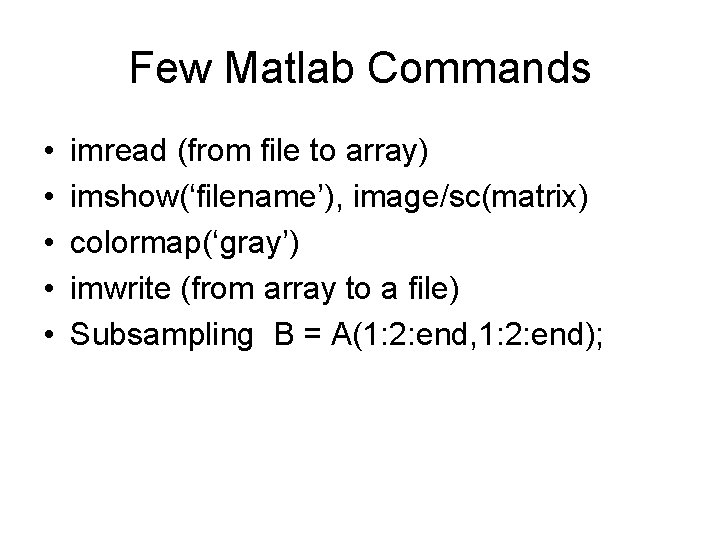
Few Matlab Commands • • • imread (from file to array) imshow(‘filename’), image/sc(matrix) colormap(‘gray’) imwrite (from array to a file) Subsampling B = A(1: 2: end, 1: 2: end);