Introduction to the Calculus and Functional Programming Languages

Introduction to the λ-Calculus and Functional Programming Languages Arne Kutzner Hanyang University 2018

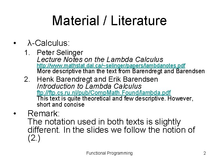
Material / Literature • λ-Calculus: 1. Peter Selinger Lecture Notes on the Lambda Calculus http: //www. mathstat. dal. ca/~selinger/papers/lambdanotes. pdf More descriptive than the text from Barendregt and Barendsen 2. Henk Barendregt and Erik Barendsen Introduction to Lambda Calculus ftp: //ftp. cs. ru. nl/pub/Comp. Math. Found/lambda. pdf This text is quite theoretical and few descriptive. However, short and concise • Remark: The notation used in both texts is slightly different. In the slides we follow the notion of (2. ) Functional Programming 2

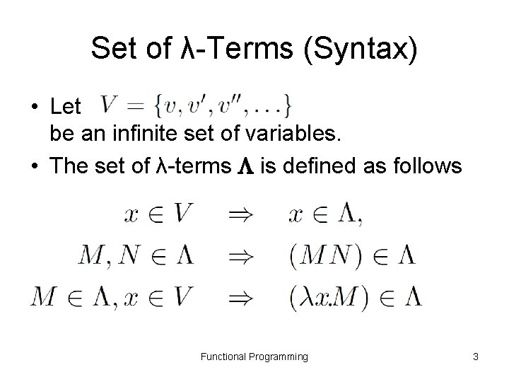
Set of λ-Terms (Syntax) • Let be an infinite set of variables. • The set of λ-terms is defined as follows Functional Programming 3

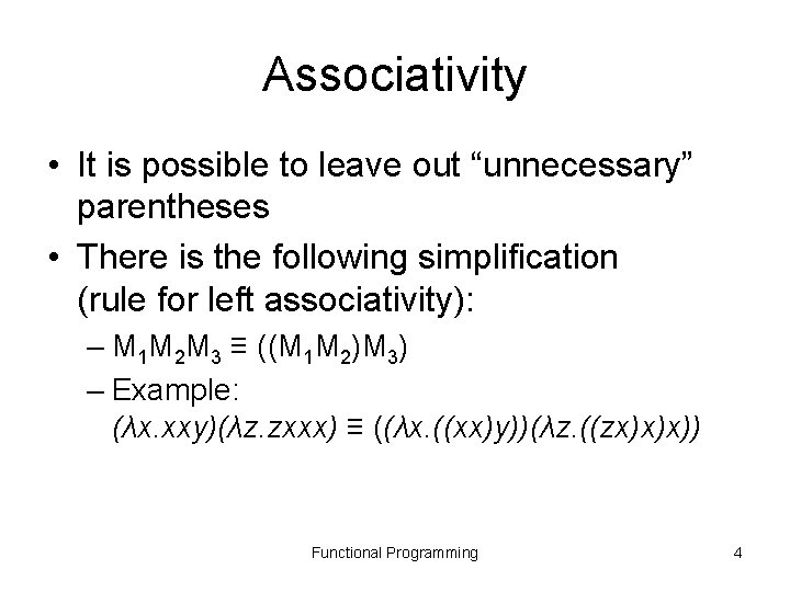
Associativity • It is possible to leave out “unnecessary” parentheses • There is the following simplification (rule for left associativity): – M 1 M 2 M 3 ≡ ((M 1 M 2)M 3) – Example: (λx. xxy)(λz. zxxx) ≡ ((λx. ((xx)y))(λz. ((zx)x)x)) Functional Programming 4

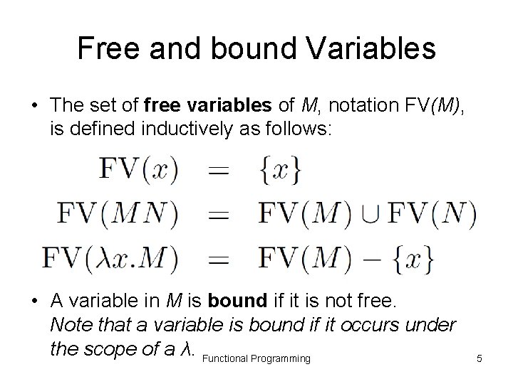
Free and bound Variables • The set of free variables of M, notation FV(M), is defined inductively as follows: • A variable in M is bound if it is not free. Note that a variable is bound if it occurs under the scope of a λ. Functional Programming 5

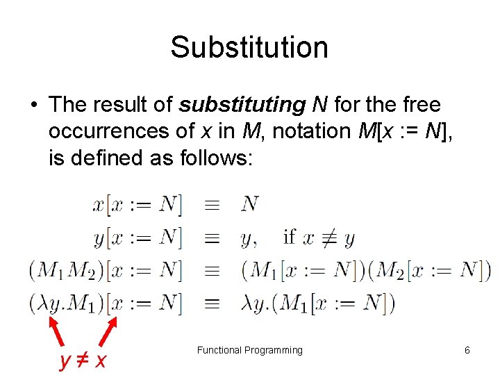
Substitution • The result of substituting N for the free occurrences of x in M, notation M[x : = N], is defined as follows: y ≠ x Functional Programming 6

Substitution (cont. ) • In the case the substitution process does not continue inside M 1 – x represents a bound variable inside M 1 • Example: bound free ((λx. xy)x(λz. z))[x: =(λa. a)] ≡ ((λx. xy)(λa. a)(λz. z)) Functional Programming 7

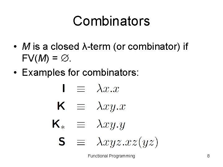
Combinators • M is a closed λ-term (or combinator) if FV(M) = . • Examples for combinators: Functional Programming 8

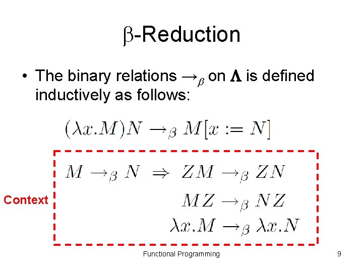
-Reduction • The binary relations → on is defined inductively as follows: Context Functional Programming 9

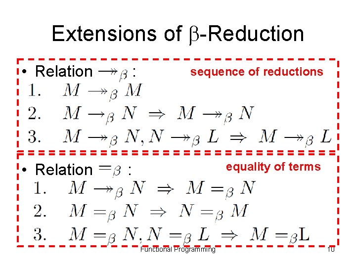
Extensions of -Reduction • Relation : sequence of reductions equality of terms : Functional Programming 10

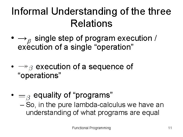
Informal Understanding of the three Relations • → single step of program execution / execution of a single “operation” • execution of a sequence of “operations” • equality of “programs” – So, in the pure lambda-calculus we have an understanding of what programs are equal Functional Programming 11

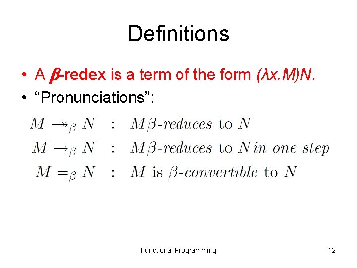
Definitions • A -redex is a term of the form (λx. M)N. • “Pronunciations”: Functional Programming 12

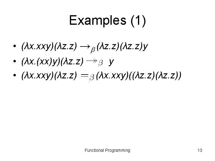
Examples (1) • (λx. xxy)(λz. z) → (λz. z)y • (λx. (xx)y)(λz. z) y • (λx. xxy)(λz. z) (λx. xxy)((λz. z)) Functional Programming 13

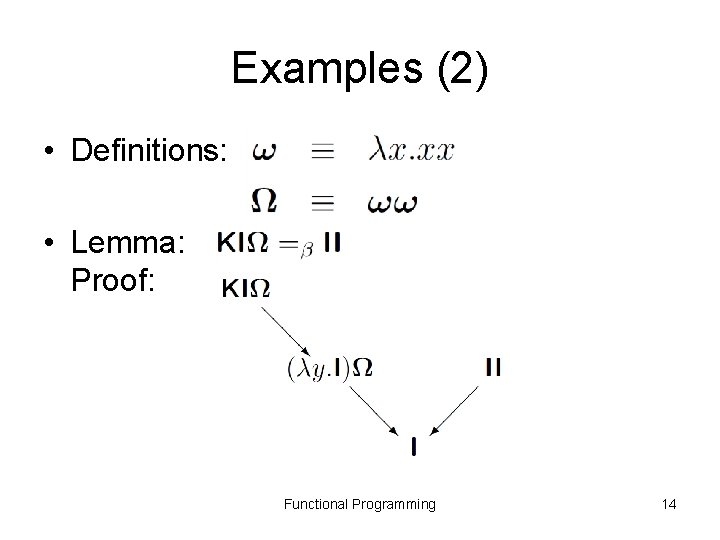
Examples (2) • Definitions: • Lemma: Proof: Functional Programming 14

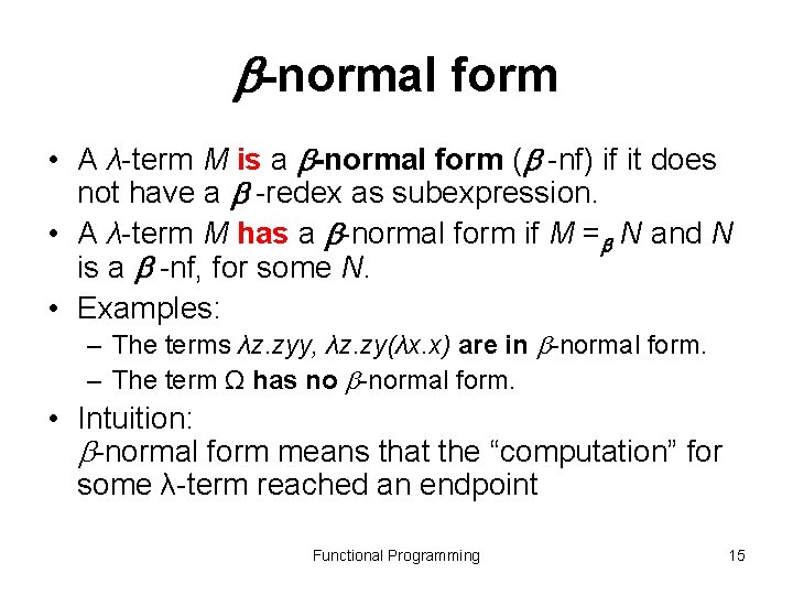
-normal form • A λ-term M is a -normal form ( -nf) if it does not have a -redex as subexpression. • A λ-term M has a -normal form if M = N and N is a -nf, for some N. • Examples: – The terms λz. zyy, λz. zy(λx. x) are in -normal form. – The term Ω has no -normal form. • Intuition: -normal form means that the “computation” for some λ-term reached an endpoint Functional Programming 15

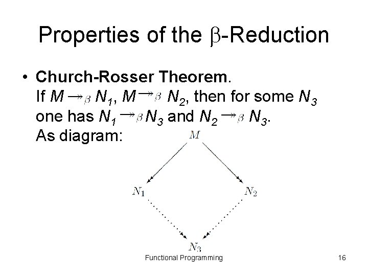
Properties of the -Reduction • Church-Rosser Theorem. If M N 1, M N 2, then for some N 3 one has N 1 N 3 and N 2 N 3. As diagram: Functional Programming 16

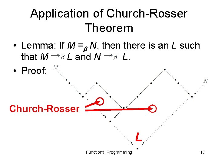
Application of Church-Rosser Theorem • Lemma: If M = N, then there is an L such that M L and N L. • Proof: Church-Rosser L Functional Programming 17

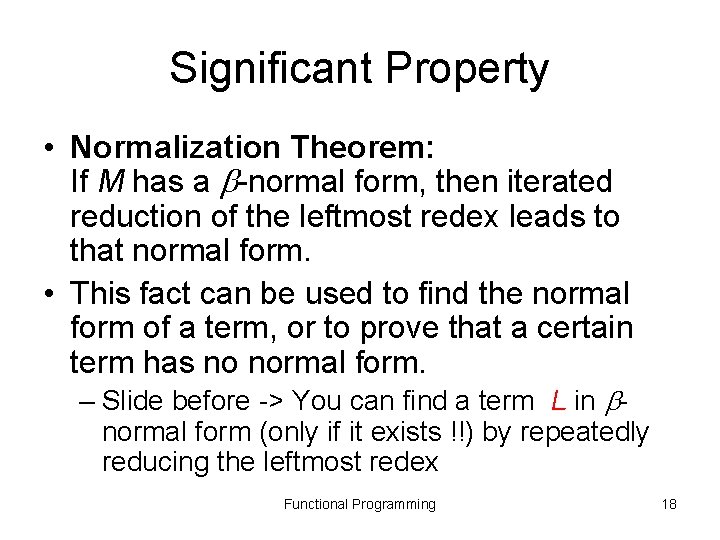
Significant Property • Normalization Theorem: If M has a -normal form, then iterated reduction of the leftmost redex leads to that normal form. • This fact can be used to find the normal form of a term, or to prove that a certain term has no normal form. – Slide before -> You can find a term L in normal form (only if it exists !!) by repeatedly reducing the leftmost redex Functional Programming 18

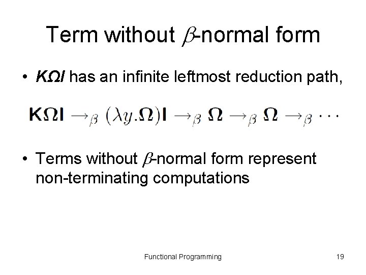
Term without -normal form • KΩI has an infinite leftmost reduction path, • Terms without -normal form represent non-terminating computations Functional Programming 19

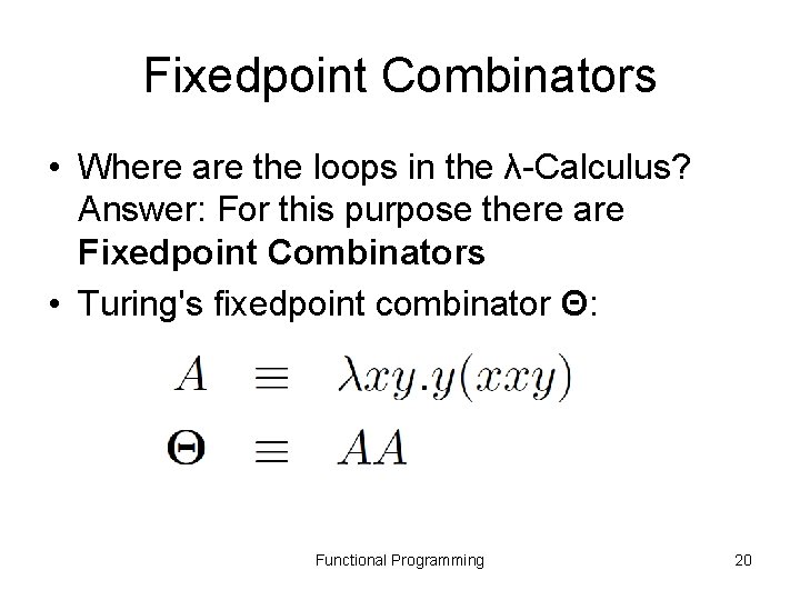
Fixedpoint Combinators • Where are the loops in the λ-Calculus? Answer: For this purpose there are Fixedpoint Combinators • Turing's fixedpoint combinator Θ: Functional Programming 20

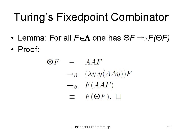
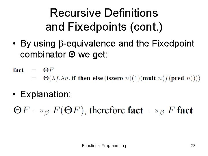
Turing’s Fixedpoint Combinator • Lemma: For all F one has ΘF F(ΘF) • Proof: Functional Programming 21

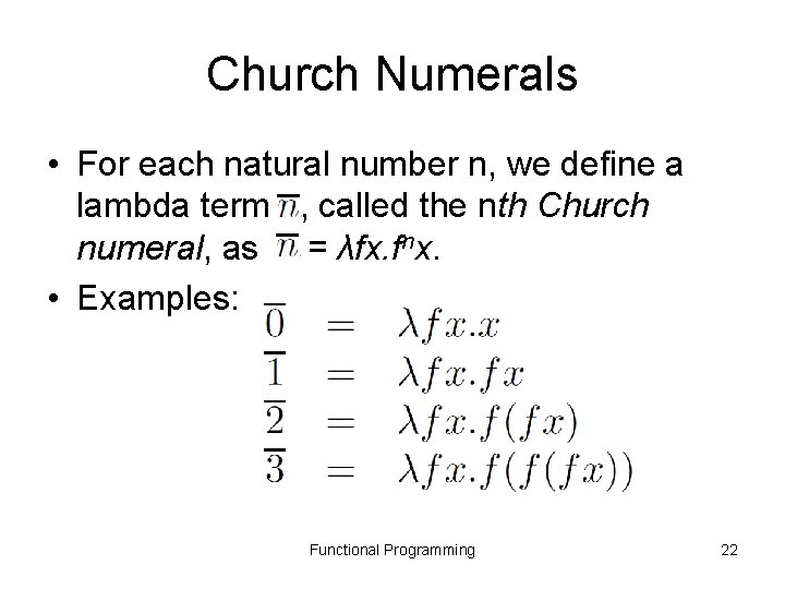
Church Numerals • For each natural number n, we define a lambda term , called the nth Church numeral, as = λfx. fnx. • Examples: Functional Programming 22

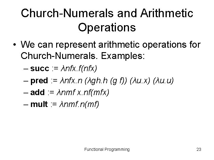
Church-Numerals and Arithmetic Operations • We can represent arithmetic operations for Church-Numerals. Examples: – succ : = λnfx. f(nfx) – pred : = λnfx. n (λgh. h (g f)) (λu. x) (λu. u) – add : = λnmf x. nf(mfx) – mult : = λnmf. n(mf) Functional Programming 23

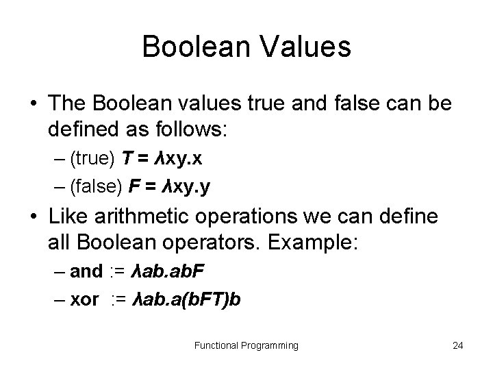
Boolean Values • The Boolean values true and false can be defined as follows: – (true) T = λxy. x – (false) F = λxy. y • Like arithmetic operations we can define all Boolean operators. Example: – and : = λab. F – xor : = λab. a(b. FT)b Functional Programming 24

Branching / if-then-else • We define: if_then_else = λx. x • We have: Functional Programming 25

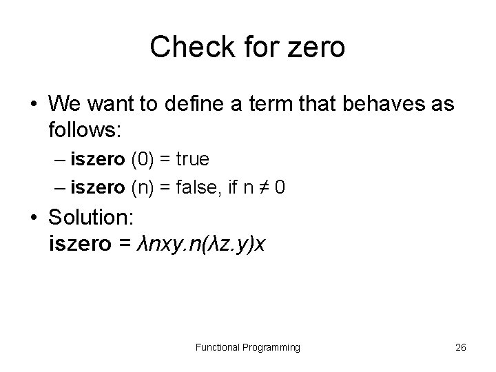
Check for zero • We want to define a term that behaves as follows: – iszero (0) = true – iszero (n) = false, if n ≠ 0 • Solution: iszero = λnxy. n(λz. y)x Functional Programming 26

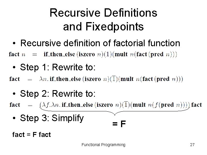
Recursive Definitions and Fixedpoints • Recursive definition of factorial function • Step 1: Rewrite to: • Step 2: Rewrite to: • Step 3: Simplify =F fact = F fact Functional Programming 27

Recursive Definitions and Fixedpoints (cont. ) • By using -equivalence and the Fixedpoint combinator Θ we get: • Explanation: Functional Programming 28

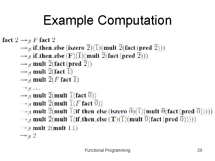
Example Computation Functional Programming 29

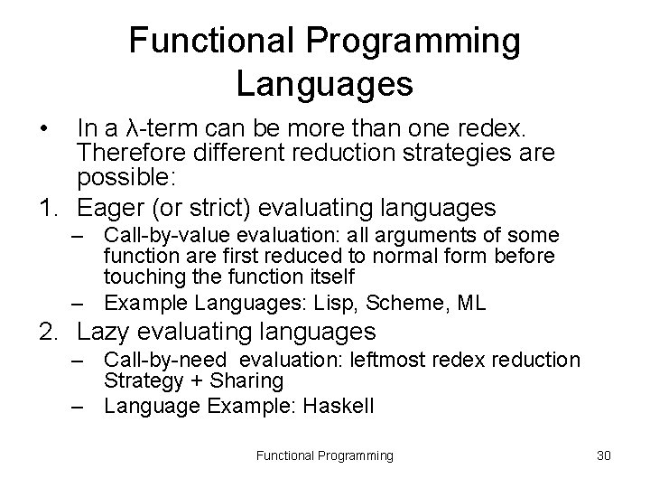
Functional Programming Languages • In a λ-term can be more than one redex. Therefore different reduction strategies are possible: 1. Eager (or strict) evaluating languages – Call-by-value evaluation: all arguments of some function are first reduced to normal form before touching the function itself – Example Languages: Lisp, Scheme, ML 2. Lazy evaluating languages – Call-by-need evaluation: leftmost redex reduction Strategy + Sharing – Language Example: Haskell Functional Programming 30

Haskell / Literature • Tutorial: Hal Daum´e III Yet Another Haskell Tutorial http: //www. cs. utah. edu/~hal/docs/daume 02 yaht. pdf • Haskell Interpreter (for exercising): Hugs / Download link: https: //www. haskell. org/hugs/pages/downloading. htm Functional Programming 31

Concepts of Functional Programming Languages • • Lists, list constructor Pattern-Matching Recursive Function Definitions Let bindings n-Tuples Polymorphism Type-Inference Input-Output Functional Programming 32

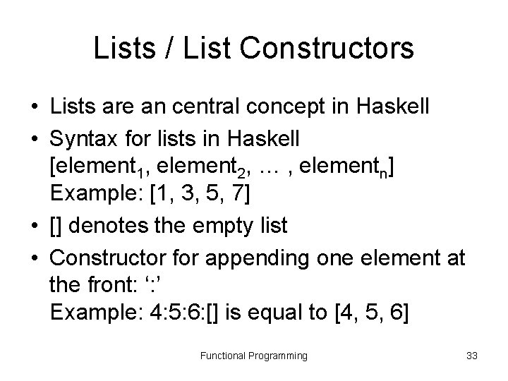
Lists / List Constructors • Lists are an central concept in Haskell • Syntax for lists in Haskell [element 1, element 2, … , elementn] Example: [1, 3, 5, 7] • [] denotes the empty list • Constructor for appending one element at the front: ‘: ’ Example: 4: 5: 6: [] is equal to [4, 5, 6] Functional Programming 33

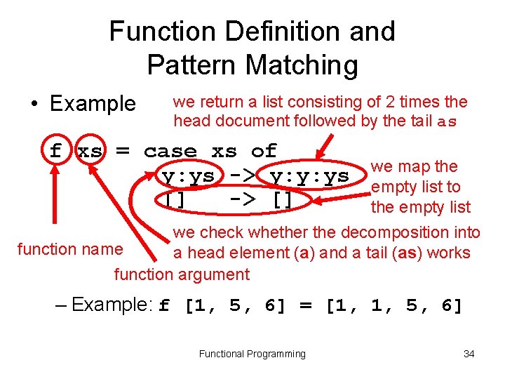
Function Definition and Pattern Matching • Example we return a list consisting of 2 times the head document followed by the tail as f xs = case xs of y: ys -> y: y: ys [] -> [] we map the empty list to the empty list we check whether the decomposition into function name a head element (a) and a tail (as) works function argument – Example: f [1, 5, 6] = [1, 1, 5, 6] Functional Programming 34

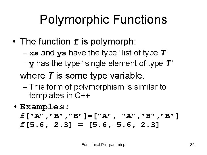
Polymorphic Functions • The function f is polymorph: – xs and ys have the type “list of type T” – y has the type “single element of type T” where T is some type variable. – This form of polymorphism is similar to templates in C++ • Examples: f["A", "B"]=["A", "B", "B"] f[5. 6, 2. 3] = [5. 6, 2. 3] Functional Programming 35

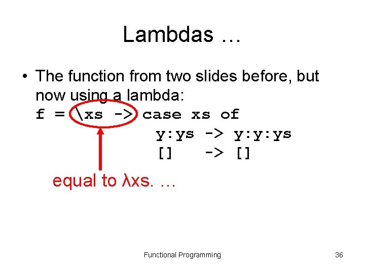
Lambdas … • The function from two slides before, but now using a lambda: f = xs -> case xs of y: ys -> y: y: ys [] -> [] equal to λxs. … Functional Programming 36

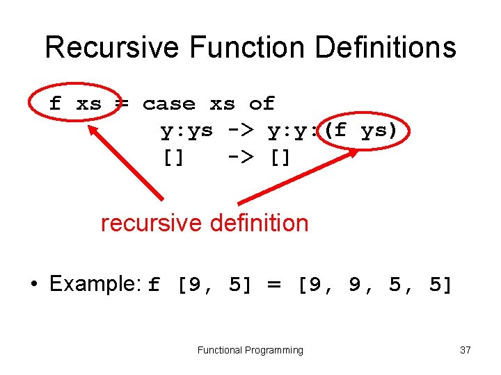
Recursive Function Definitions f xs = case xs of y: ys -> y: y: (f ys) [] -> [] recursive definition • Example: f [9, 5] = [9, 9, 5, 5] Functional Programming 37

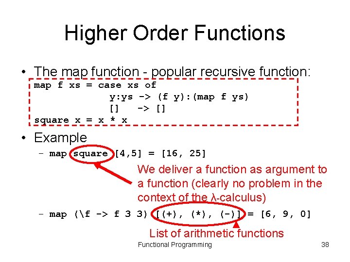
Higher Order Functions • The map function - popular recursive function: map f xs = case xs of y: ys -> (f y): (map f ys) [] -> [] square x = x * x • Example – map square [4, 5] = [16, 25] We deliver a function as argument to a function (clearly no problem in the context of the λ-calculus) – map (f -> f 3 3) [(+), (*), (-)] = [6, 9, 0] List of arithmetic functions Functional Programming 38

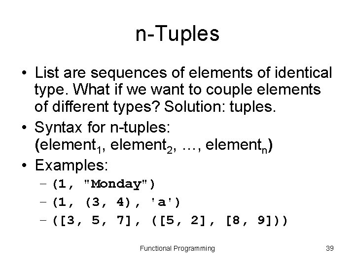
n-Tuples • List are sequences of elements of identical type. What if we want to couple elements of different types? Solution: tuples. • Syntax for n-tuples: (element 1, element 2, …, elementn) • Examples: – (1, "Monday") – (1, (3, 4), 'a') – ([3, 5, 7], ([5, 2], [8, 9])) Functional Programming 39

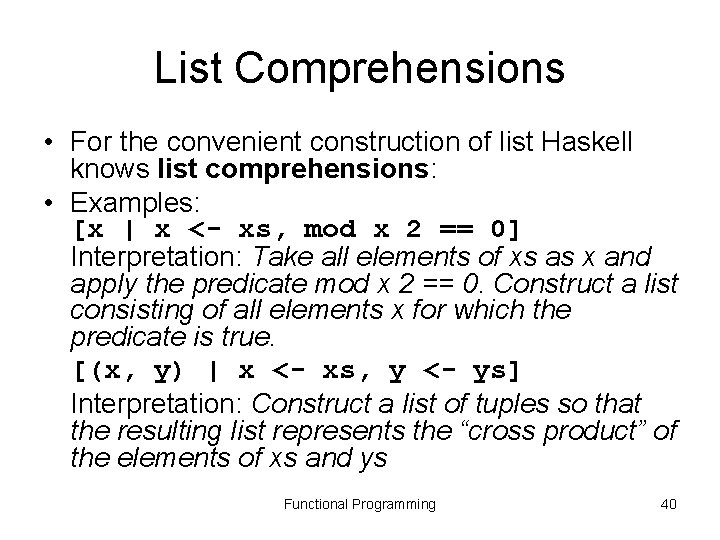
List Comprehensions • For the convenient construction of list Haskell knows list comprehensions: • Examples: [x | x <- xs, mod x 2 == 0] Interpretation: Take all elements of xs as x and apply the predicate mod x 2 == 0. Construct a list consisting of all elements x for which the predicate is true. [(x, y) | x <- xs, y <- ys] Interpretation: Construct a list of tuples so that the resulting list represents the “cross product” of the elements of xs and ys Functional Programming 40

Quicksort in Haskell (using list comprehensions) • Possible implementation of Quicksort [] = [] sort (x: xs) = sort [s | s <- xs, s <= x] ++ x: sort [s | s <- xs, s > x] pivot element list concatenation pattern matching like in a case-clause Functional Programming 41

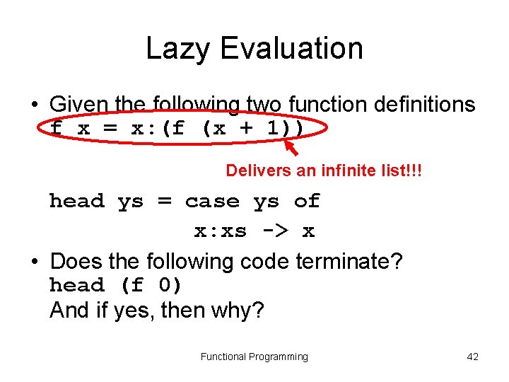
Lazy Evaluation • Given the following two function definitions f x = x: (f (x + 1)) Delivers an infinite list!!! head ys = case ys of x: xs -> x • Does the following code terminate? head (f 0) And if yes, then why? Functional Programming 42

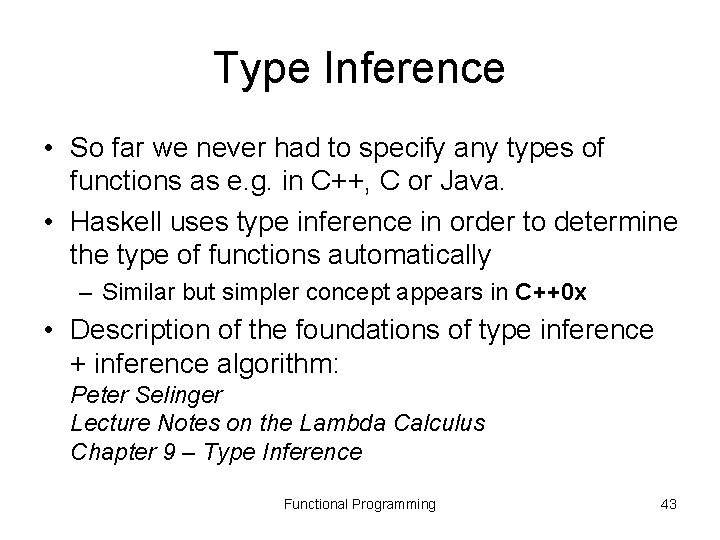
Type Inference • So far we never had to specify any types of functions as e. g. in C++, C or Java. • Haskell uses type inference in order to determine the type of functions automatically – Similar but simpler concept appears in C++0 x • Description of the foundations of type inference + inference algorithm: Peter Selinger Lecture Notes on the Lambda Calculus Chapter 9 – Type Inference Functional Programming 43

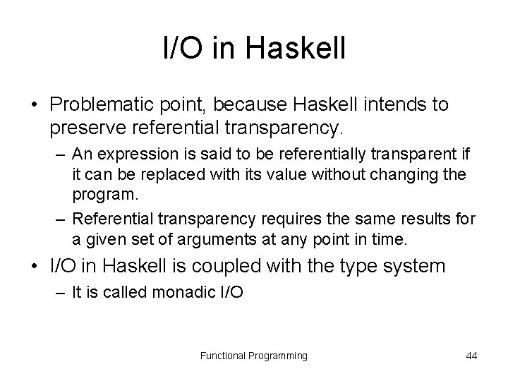
I/O in Haskell • Problematic point, because Haskell intends to preserve referential transparency. – An expression is said to be referentially transparent if it can be replaced with its value without changing the program. – Referential transparency requires the same results for a given set of arguments at any point in time. • I/O in Haskell is coupled with the type system – It is called monadic I/O Functional Programming 44

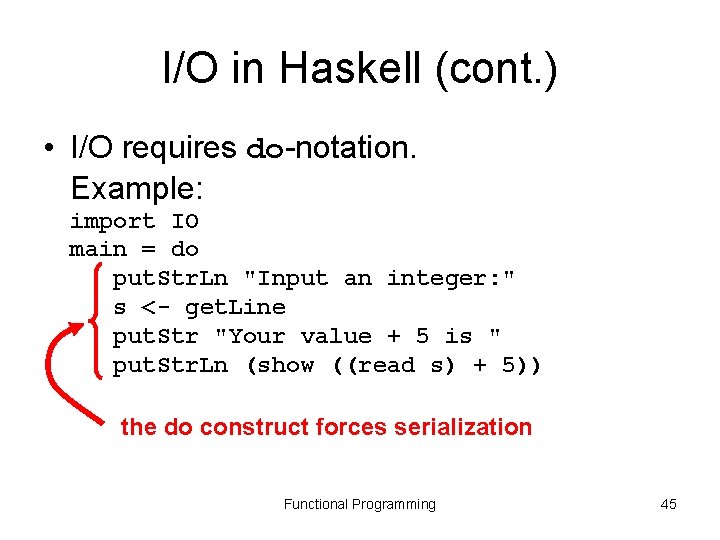
I/O in Haskell (cont. ) • I/O requires do-notation. Example: import IO main = do put. Str. Ln "Input an integer: " s <- get. Line put. Str "Your value + 5 is " put. Str. Ln (show ((read s) + 5)) the do construct forces serialization Functional Programming 45