Introduction to stellar reaction rates Nuclear reactions generate

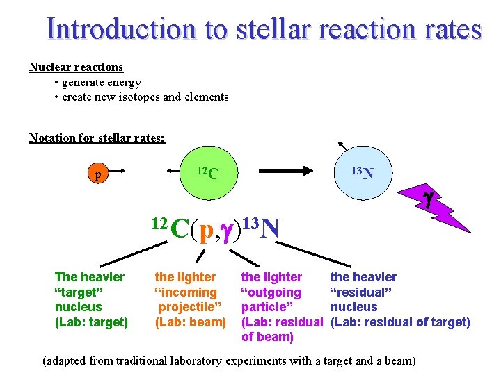
Introduction to stellar reaction rates Nuclear reactions • generate energy • create new isotopes and elements Notation for stellar rates: p 12 C 13 N g 12 C(p, g)13 N The heavier “target” nucleus (Lab: target) the lighter “incoming projectile” (Lab: beam) the lighter “outgoing particle” (Lab: residual of beam) the heavier “residual” nucleus (Lab: residual of target) (adapted from traditional laboratory experiments with a target and a beam)

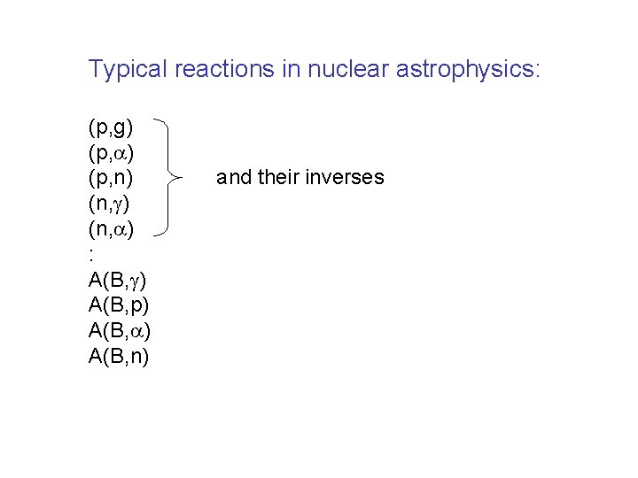
Typical reactions in nuclear astrophysics: (p, g) (p, a) (p, n) (n, g) (n, a) : A(B, g) A(B, p) A(B, a) A(B, n) and their inverses

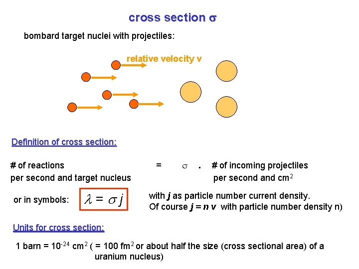
cross section s bombard target nuclei with projectiles: relative velocity v Definition of cross section: # of reactions per second and target nucleus or in symbols: l=sj = . # of incoming projectiles per second and cm 2 with j as particle number current density. Of course j = n v with particle number density n) Units for cross section: 1 barn = 10 -24 cm 2 ( = 100 fm 2 or about half the size (cross sectional area) of a uranium nucleus)

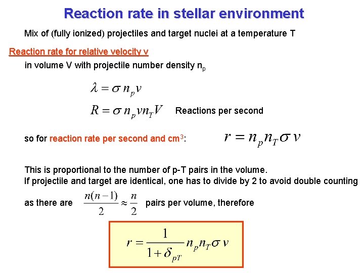
Reaction rate in stellar environment Mix of (fully ionized) projectiles and target nuclei at a temperature T Reaction rate for relative velocity v in volume V with projectile number density np Reactions per second so for reaction rate per second and cm 3: This is proportional to the number of p-T pairs in the volume. If projectile and target are identical, one has to divide by 2 to avoid double counting as there are pairs per volume, therefore

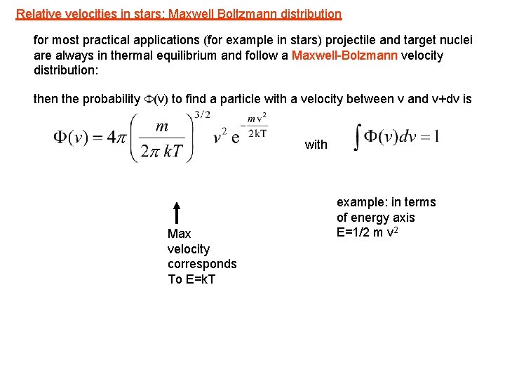
Relative velocities in stars: Maxwell Boltzmann distribution for most practical applications (for example in stars) projectile and target nuclei are always in thermal equilibrium and follow a Maxwell-Bolzmann velocity distribution: then the probability F(v) to find a particle with a velocity between v and v+dv is with Max velocity corresponds To E=k. T example: in terms of energy axis E=1/2 m v 2

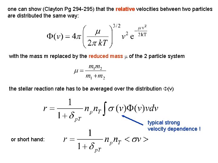
one can show (Clayton Pg 294 -295) that the relative velocities between two particles are distributed the same way: with the mass m replaced by the reduced mass m of the 2 particle system the stellar reaction rate has to be averaged over the distribution F(v) typical strong velocity dependence ! or short hand:

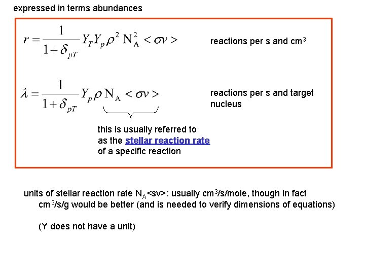
expressed in terms abundances reactions per s and cm 3 reactions per s and target nucleus this is usually referred to as the stellar reaction rate of a specific reaction units of stellar reaction rate NA<sv>: usually cm 3/s/mole, though in fact cm 3/s/g would be better (and is needed to verify dimensions of equations) (Y does not have a unit)

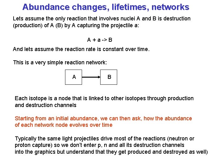
Abundance changes, lifetimes, networks Lets assume the only reaction that involves nuclei A and B is destruction (production) of A (B) by A capturing the projectile a: A + a -> B And lets assume the reaction rate is constant over time. This is a very simple reaction network: A B Each isotope is a node that is linked to other isotopes through production and destruction channels Starting from an initial abundance, we can then ask, how the abundance of each network node evolves over time Typically the same light projectiles drive most of the reactions (neutron or proton capture) so we don’t enter p, n and all its destruction channels into the graphics but understand that they get produced and destroyed as well)

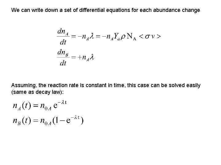
We can write down a set of differential equations for each abundance change Assuming, the reaction rate is constant in time, this case can be solved easily (same as decay law):

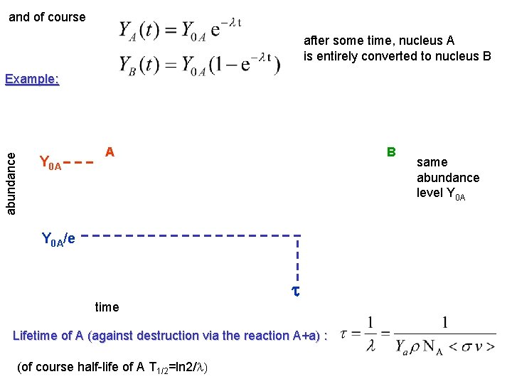
and of course after some time, nucleus A is entirely converted to nucleus B abundance Example: Y 0 A A B Y 0 A/e time t Lifetime of A (against destruction via the reaction A+a) : (of course half-life of A T 1/2=ln 2/l) same abundance level Y 0 A

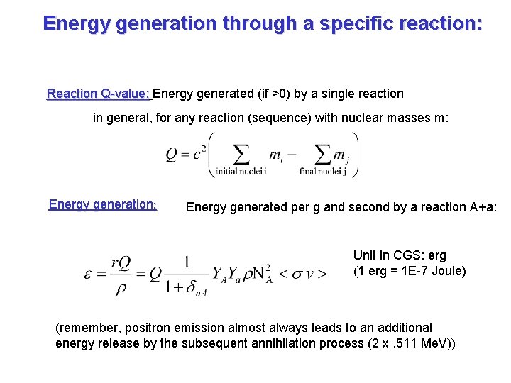
Energy generation through a specific reaction: Reaction Q-value: Energy generated (if >0) by a single reaction in general, for any reaction (sequence) with nuclear masses m: Energy generation: Energy generated per g and second by a reaction A+a: Unit in CGS: erg (1 erg = 1 E-7 Joule) (remember, positron emission almost always leads to an additional energy release by the subsequent annihilation process (2 x. 511 Me. V))

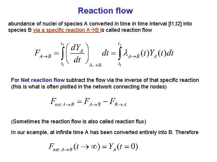
Reaction flow abundance of nuclei of species A converted in time interval [t 1, t 2] into species B via a specific reaction A B is called reaction flow For Net reaction flow subtract the flow via the inverse of that specific reaction (this is what is often plotted in the network connecting the nodes) (Sometimes the reaction flow is also called reaction flux) In our example, at infinite time A has been converted entirely into B. Therefore

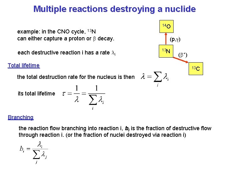
Multiple reactions destroying a nuclide example: in the CNO cycle, 13 N can either capture a proton or b decay. each destructive reaction i has a rate li Total lifetime 14 O (p, g) 13 N (b+) 13 C the total destruction rate for the nucleus is then its total lifetime Branching the reaction flow branching into reaction i, bi is the fraction of destructive flow through reaction i. (or the fraction of nuclei destroyed via reaction i)

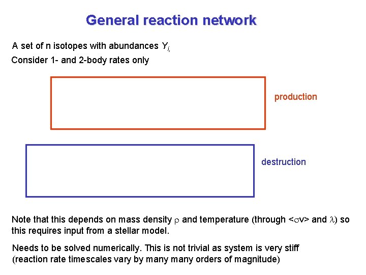
General reaction network A set of n isotopes with abundances Yi, Consider 1 - and 2 -body rates only production destruction Note that this depends on mass density r and temperature (through < v> and l) so this requires input from a stellar model. Needs to be solved numerically. This is not trivial as system is very stiff (reaction rate timescales vary by many orders of magnitude)

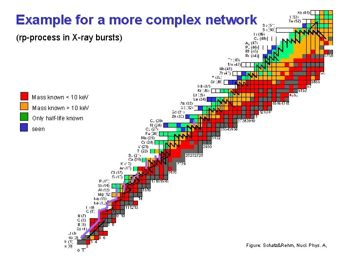
Example for a more complex network (rp-process in X-ray bursts) Mass known < 10 ke. V Mass known > 10 ke. V Only half-life known seen Figure: Schatz&Rehm, Nucl. Phys. A,