Introduction to Statistics for the Social Sciences SBS

Introduction to Statistics for the Social Sciences SBS 200 - Lecture Section 001, Spring 2018 Room 150 Harvill Building 9: 00 - 9: 50 Mondays, Wednesdays & Fridays. 4/23/18

Screen Lecturer’s desk Row A Row B Row F 3 12 11 10 9 8 7 6 5 4 Row A 2 1 5 4 3 2 Row B 19 24 23 22 21 Row C 20 19 18 17 16 15 14 13 12 11 10 9 8 7 6 5 4 3 2 28 27 26 25 24 23 Row D 22 21 20 19 18 17 16 15 14 13 12 11 10 9 8 7 6 5 4 3 2 1 30 29 28 27 26 25 24 23 Row E 23 22 21 20 19 18 17 16 15 14 13 12 11 10 9 8 7 6 5 4 3 2 1 Row D 31 13 22 21 20 Row C Row E Row A 15 14 29 25 23 18 17 16 15 14 13 12 11 10 9 8 7 6 1 Row B 1 Row C Row D Row E 35 34 33 32 31 30 29 28 27 26 Row F 25 24 23 22 21 20 19 18 17 16 15 14 13 12 11 10 9 8 7 6 5 4 3 2 1 Row F 35 34 33 32 31 30 29 28 27 26 Row G 25 24 23 22 21 20 19 18 17 16 15 14 13 12 11 10 9 8 7 6 5 4 3 2 1 Row G 37 36 35 34 33 32 31 30 29 28 Row H 27 26 25 24 23 22 21 20 19 18 17 16 15 14 13 12 41 40 39 38 37 36 35 34 33 32 31 30 29 Row J 28 27 26 25 24 23 22 21 20 19 18 17 16 15 14 13 12 11 10 9 8 7 6 5 4 3 2 1 Row J 41 40 39 38 37 36 35 34 33 32 31 30 29 Row K 28 27 26 25 24 23 22 21 20 19 18 17 16 15 14 13 12 11 10 9 8 7 6 5 4 3 2 1 Row K 25 Row L 24 23 22 21 20 19 18 17 16 15 14 13 12 11 10 9 20 19 Row M 18 17 16 15 14 13 12 11 10 9 8 7 6 5 4 3 Row N 15 14 13 12 11 10 9 8 7 6 5 4 3 2 1 Row P 15 14 13 12 11 10 9 8 7 6 5 4 3 2 1 Row G Row H Row L 33 32 31 30 29 28 27 26 Row M 21 table 15 14 13 12 11 10 9 8 7 6 Projection Booth 5 4 3 2 1 11 10 9 8 7 6 5 4 3 2 2 1 1 1 Row L Row M Harvill 150 renumbered Left handed desk Row H

 Open.")
Schedule of readings Before our fourth and final exam (April 30 th) Open. Stax Chapters 1 – 13 (Chapter 12 is emphasized) Plous Chapter 17: Social Influences Chapter 18: Group Judgments and Decisions

k. e Project w 4 eek e w s i h al t eview. n o i t p Due this o r be 4 l l i w m a s x b E La on s u c o f l Wil
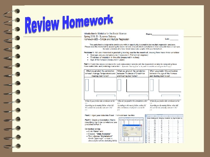

0 20 40 60 80 Average Temperature Heating Cost 500 400 300 200 100 0 20 40 60 Insulation 80 500 400 300 200 100 0 20 40 60 80 Age of Furnace r(18) = - 0. 50 r(18) = - 0. 40 r(18) = + 0. 60 r(18) = - 0. 811508835 r(18) = - 0. 257101335 r(18) = + 0. 536727562

0 20 40 60 80 Average Temperature Heating Cost 500 400 300 200 100 0 20 40 60 Insulation 80 500 400 300 200 100 0 20 40 60 80 Age of Furnace r(18) = - 0. 50 r(18) = - 0. 40 r(18) = + 0. 60 r(18) = - 0. 811508835 r(18) = - 0. 257101335 r(18) = + 0. 536727562

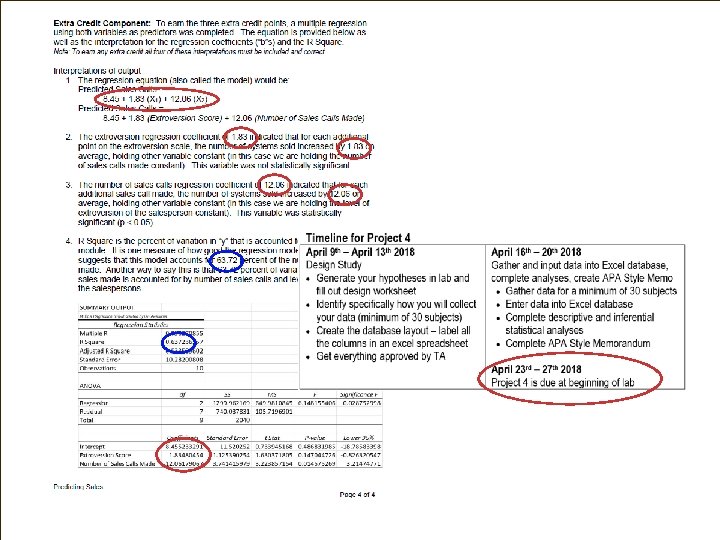
+ 427. 19 - 4. 5827 -14. 8308 + 6. 1010 Y’ = 427. 19 - 4. 5827 x 1 - 14. 8308 x 2 + 6. 1010 x 3

+ 427. 19 - 4. 5827 -14. 8308 + 6. 1010 Y’ = 427. 19 - 4. 5827 x 1 - 14. 8308 x 2 + 6. 1010 x 3

+ 427. 19 - 4. 5827 -14. 8308 + 6. 1010 Y’ = 427. 19 - 4. 5827 x 1 - 14. 8308 x 2 + 6. 1010 x 3

+ 427. 19 - 4. 5827 -14. 8308 + 6. 1010 Y’ = 427. 19 - 4. 5827 x 1 - 14. 8308 x 2 + 6. 1010 x 3

+ 427. 19 - 4. 5827 -14. 8308 + 6. 1010 Y’ = 427. 19 - 4. 5827 x 1 - 14. 8308 x 2 + 6. 1010 x 3
-14. 8308")
4. 58 14. 83 6. 10 Y’ = 427. 19 - 4. 5827(30)-14. 8308 (5) +6. 1010 (10) Y’ = 427. 19 - 137. 481 - 74. 154 + 61. 010 = $ 276. 56 Calculate the predicted heating cost using the new value for the age of the furnace Use the regression coefficient for the furnace ($6. 10), to estimate the change
-14. 8308")
4. 58 14. 83 6. 10 Y’ = 427. 19 - 4. 5827(30)-14. 8308 (5) +6. 1010 (10) Y’ = 427. 19 - 137. 481 - 74. 154 + 61. 010 = $ 276. 56 Y’ = 427. 19 - 4. 5827(30)-14. 8308 (5) +6. 1010 (10) These differ by only one Y’ = $427. 19 year but heating cost 276. 56 - 137. 481 - 74. 154 + 61. 010 = $ 276. 56 Y’ = 427. 19 - 4. 5827(30)-14. 8308 (5) +6. 1010 (11) Y’ = 427. 19 - 137. 481 - 74. 154 + 67. 111 = $ 282. 66 changed by $6. 10 282. 66 – 276. 56 = 6. 10 Calculate the predicted heating cost using the new value for the age of the furnace Use the regression coefficient for the furnace ($6. 10), to estimate the change

4. 0 3. 0 2. 0 1. 0 GPA 4. 0 2. 0 1. 0 0 1 2 3 4 High School GPA 2. 0 1. 0 0 200 300 400 500 600 SAT (Verbal) 0 200 300 400 500 600 SAT (Mathematical) r(7) = 0. 50 r(7) = + 0. 80 r(7) = + 0. 911444123 r(7) = + 0. 616334867 r(7) = + 0. 487295007

4. 0 3. 0 2. 0 1. 0 GPA 4. 0 2. 0 1. 0 0 1 2 3 4 High School GPA 2. 0 1. 0 0 200 300 400 500 600 SAT (Verbal) 0 200 300 400 500 600 SAT (Mathematical) r(7) = 0. 50 r(7) = + 0. 80 r(7) = + 0. 911444123 r(7) = + 0. 616334867 r(7) = + 0. 487295007

4. 0 3. 0 2. 0 1. 0 GPA 4. 0 2. 0 1. 0 0 1 2 3 4 High School GPA 2. 0 1. 0 0 200 300 400 500 600 SAT (Verbal) 0 200 300 400 500 600 SAT (Mathematical) r(7) = 0. 50 r(7) = + 0. 80 r(7) = + 0. 911444123 r(7) = + 0. 616334867 r(7) = + 0. 487295007

4. 0 3. 0 2. 0 1. 0 GPA 4. 0 2. 0 1. 0 0 1 2 3 4 High School GPA 2. 0 1. 0 0 200 300 400 500 600 SAT (Verbal) 0 200 300 400 500 600 SAT (Mathematical) r(7) = 0. 50 r(7) = + 0. 80 r(7) = + 0. 911444123 r(7) = + 0. 616334867 r(7) = + 0. 487295007

- 0. 41107 No

- 0. 41107 + 1. 2013 No Yes

- 0. 41107 + 1. 2013 0. 0016 No Yes No

- 0. 41107 + 1. 2013 0. 0016 - 0. 0019 No Yes No No

- 0. 41107 + 1. 2013 0. 0016 - 0. 0019 High School GPA No Yes No No

- 0. 41107 + 1. 2013 0. 0016 - 0. 0019 High School GPA Y’ = - 0. 41107 + 1. 2013 x 1+ 0. 0016 x 2 - 0. 0019 x 3 No Yes No No

1. 201. 0016. 0019 Y’ = - 0. 41107 + 1. 2013 x 1+ 0. 0016 x 2 - 0. 0019 x 3 Y’ = - 0. 411+ 1. 2013 (2. 8)+ 0. 0016 (430) - 0. 0019 (460) = 2. 76

1. 201. 0016. 0019 Y’ = - 0. 41107 + 1. 2013 x 1+ 0. 0016 x 2 - 0. 0019 x 3 Y’ = - 0. 411+ 1. 2013 (3. 8)+ 0. 0016 (430) - 0. 0019 (460) = 3. 96

1. 201. 0016. 0019 2. 76 3. 96 - 2. 76 = 1. 2 Yes, use the regression coefficient for the HS GPA (1. 2), to estimate the change

Let’s try one When using hypothesis testing for correlation, Correct what is our null hypothesis? a. There is no relationship between the variables (r = 0) b. There is a relationship between the variables (r ≠ 0) c. Not enough info is given

Let’s try one When using hypothesis testing for correlation, if we reject the null, what are we concluding? a. There is no relationship between the variables (r = 0) b. There is a relationship between the variables (r ≠ 0) c. Not enough info is given Correct

Let’s try one Winnie found an observed correlation coefficient of 0, what should she conclude? a. Reject the null hypothesis b. Do not reject the null hypothesis Correct c. Not enough info is given

In the regression equation, what does the letter "a" represent? a. Y intercept Correct b. Slope of the line c. Any value of the independent variable that is selected d. None of these Y’ = a + bx 1 + bx 2 + bx 3 + bx 4

Assume the least squares equation is Y’ = 10 + 20 X. What does the value of 10 in the equation indicate? a. Y intercept Correct b. For each unit increased in Y, X increases by 10 c. For each unit increased in X, Y increases by 10 d. None of these.

In the least squares equation, Y’ = 10 + 20 X the value of 20 indicates a. the Y intercept. b slope (so for each unit increase in X, Y’ increases by 20). c. slope (so for each unit increase in Y’, X increases by 20). Correct d. none of these.

In the equation Y’ = a + b. X, what is Y’ ? a. Slope of the line b. Y intercept C. Predicted value of Y, given a specific X value d. Value of Y when X = 0 Correct

If there are four independent variables in a multiple regression equation, there also four a. Y-intercepts (a). b. regression coefficients (slopes or bs). Correct c. dependent variables. d. constant terms (k). Y’ = a + bx 1 + bx 2 + bx 3 + bx 4

According to the Central Limit Theorem, which is false? a. As n ↑ x will approach µ b. As n ↑ curve will approach normal shape c. As n ↑ curve variability gets larger d. As n ↑ Correct

What is the null hypothesis of a correlation coefficient? a. It is zero (nothing going on) Correct b. It is less than zero c. It is more than zero d. It equals the computed sample correlation

Let’s try one Winnie found an observed correlation coefficient of 0, what should she conclude? a. Reject the null hypothesis b. Do not reject the null hypothesis Correct c. Not enough info is given

If the coefficient of determination is 0. 80, what percent of variation is explained? a. 20% b. 90% c. 64% Correct d. 80% coefficient of determination = r 2 What percent of variation is not explained? a. 20% Correct b. 90% c. 64% d. 80%

Which of the following represents a significant finding: a. p < 0. 05 Correct b. t(3) = 0. 23; n. s. c. the observed t statistic is nearly zero d. we do not reject the null hypothesis

In multiple regression what is the range of values for a coefficient of regression? a. 0 to +1. 0 b. 0 to -1. 0 c. -1. 0 to +1. 0 d. Any number at all Correct Y’ = a + b 1 X 1 + b 2 X 2 + b 3 X 3

Correct If r = 1. 00, which inference cannot be made? a. The dependent variable can be perfectly predicted by the independent variable b. This provides evidence that the dependent variable is caused by the independent variable c. All of the variation in the dependent variable can be accounted for by the independent variable d. Coefficient of determination is 100%.

Let’s try one In a regression analysis what do we call the variable used to predict the value of another variable? a. Independent Correct b. Dependent c. Correlation d. Determination

What can we conclude if the coefficient of determination is 0. 94? a. r 2 = 0. 94 b. direction of relationship is positive c. 94% of total variation of one variable is explained by variation in the other variable. d. Both A and C Correct

Which of the following statements regarding the coefficient of correlation is true? a. It ranges from -1. 0 to +1. 0 b. It measures the strength of the relationship between two variables c. A value of 0. 00 indicates two variables are not related d. All of these Correct
")
What does a coefficient of correlation of 0. 70 infer? (r = +0. 70) a. Almost no correlation because 0. 70 is close to 1. 0 b. 70% of the variation in one variable is explained by the other c. Coefficient of determination is 0. 49 d. Coefficient of nondetermination is 0. 30 Correct coefficient of correlation = r coefficient of determination = r 2


go down narrower As variability goes down, it is easier to reject the null ANOVA 99. 18%

z= 52 -40 z = 2. 4 5 Go to table Add area Lower half . 4918 +. 5000 =. 9918 also fine: 99. 18%. 9918. 5000 . 4918 40 4 2. z =

go down narrower As variability goes down, it is easier to reject the null ANOVA 99. 18% 0 Interval True experiment

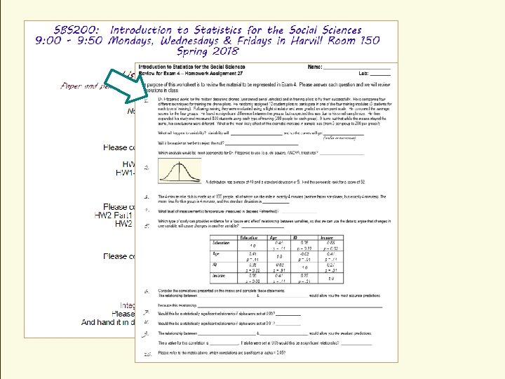
Education Income has the largest correlation coefficient of 0. 85 Yes No IQ Age No 0. 91 Income x Education is a significant correlation, p < 0. 05 None r 2

Standard error of the estimate because it is a measure of the amount of error in the regression line (average of residuals) 81% because. 92 =. 81 19% The correlation between the heights of mothers and their daughters is moderate, positive and statistically significant, r(28) = 0. 60; p< 0. 05 36% because. 62 =. 36 64% because so 36% is explained so 64% is not explained - 100 – 36 = 64 75% because. 52 =. 25, so 25% is explained so 75% is not explained

r = 0. 92 r 2 = 0. 8464 b = 6. 0857 84. 64% 15. 36% b = 6. 0857 55. 286 b = 6. 0857 residual r b b r 2 a -1. 0 +1. 0 anything anything 0 any positive number

They are both difference from expected value Residual is difference from score to predicted score (y – y’) Deviation score is difference from score to mean (x - µ) Over-performing The standard error of the estimate is the average of the residuals just like standard deviation is the average of the deviation scores zero That there is no significant difference between these groups

1 3 480. 94 -4. 89 -14. 76 3. 06 Y’ = 480. 94 - 4. 89 (temp) - 14. 76 (insulation) + 3. 06 (age) Y’ = 480. 94 - 4. 89 x 1 - 14. 76 x 2 + 3. 06 x 3 1 3
 Decrease")
Yes Decrease variability (by increasing sample size or minimize variability due to error) Decrease level of confidence from 99% to 95% Easier Narrower Easier Common and rare scores

Get smaller Type of cartoon Two-tail 48 Level of aggression True No difference in level of aggression based on type of cartoon watched Type of cartoon did make difference in level of aggression did make a difference didn’t make a difference Mean approaches true population Shape approaches normality Variability goes down it didn’t it did

58 3 100 12 25 4. 0 3. 5 3. 49 84 percentile

58 3 100 12 25 4. 0 3. 5 3. 49 84 percentile

- Slides: 63