Introduction to Statistics for the Social Sciences SBS

Introduction to Statistics for the Social Sciences SBS 200 - Lecture Section 001, Fall 2019 Social Sciences Room 100 10: 00 - 10: 50 Mondays, Wednesdays & Fridays. December 4

 Open. Stax Chapters 1 –")
Schedule of readings Before next exam (December 9) Open. Stax Chapters 1 – 13 (Chapter 12 is emphasized) Please read Chapters 17 and 18 Plous Chapter 17: Social Influences Chapter 18: Group Judgments and Decisions Study Guide is posted

Labs Continue this week

Regression Example Rory is an owner of a small software company and employs 10 sales staff. Rory send his staff all over the world consulting, selling and setting up his system. He wants to evaluate his staff in terms of who are the most (and least) productive sales people and also whether more sales calls actually result in more systems being sold. So, he simply measures the number of sales calls made by each sales person and how many systems they successfully sold.

Regression: Evaluating Staff Step 1: Compare expected sales levels to actual sales levels Ava Isabella Madison Emma -23. 7 Joshua Jacob 14. 7 Difference between expected Y’ and actual Y is called “residual” (it’s a deviation score) Emily

Regression: Evaluating Staff Step 1: Compare expected sales levels to actual sales levels Ava Isabella Emma Emily Madison Joshua Jacob What should you expect from each salesperson They should sell x systems depending on sales calls If they sell more over performing If they sell fewer underperforming

How do we find the average amount of error in our prediction The average amount by which actual scores deviate on either side of the predicted score Residual scores Ava is 14. 7 Jacob is -23. 7 Emily is -6. 8 Madison is 7. 9 Step 1: Find error for each value (just the residuals) Y – Y’ Step 2: Add up the residuals Σ(Y – Y’) = 0 Σ(Y – Y’) 2 Square root Big problem Square the deviations Σ(Y – Y’) 2 n-2 Divide by df Difference between expected Y’ and actual Y is called “residual” (it’s a deviation score) How would we find our “average residual”? Σx N The green lines show much “error” there is in our prediction line…how much we are wrong in our predictions

How do we find the average amount of error in our prediction Deviation scores Step 1: Find error for each value (just the residuals) Y – Y’ Sound familia r? ? Step 2: Find average √ ∑(Y – Y’)2 n - 2 Diallo is 0” Preston is 2” Mike is -4” Hunter is -2 Difference between expected Y’ and actual Y is called “residual” (it’s a deviation score) How would we find our “average residual”? Σx N The green lines show much “error” there is in our prediction line…how much we are wrong in our predictions
 These would be helpful to know by")
Standard error = of the estimate (line) These would be helpful to know by heart – please memorize these formula

What is r 2? r 2 = The proportion of the total variance in the predicted variable that is explained by its relationship with the predictor variable Examples If ice cream sales and temperature are correlated with an r =. 5, then what amount (proportion or percentage) of variance of ice cream sales is accounted for by temperature? . 25 because (. 5)2 =. 25

What is r 2? r 2 = The proportion of the total variance in the predicted variable that is explained by its relationship with the predictor variable Examples If ice cream sales and temperature are correlated with an r =. 5, then what amount (proportion or percentage) of variance of ice cream sales is not accounted for by temperature? . 75 because (1. 0 -. 25) =. 75 or 75% because 100% - 25% = 75%

Interpreting regression equation Prediction line Y’ = a + b 1 X 1 The expected cost for dinner as predicted by the number of people Cost = 15. 22 + 19. 96 Persons Cost will be about 95. 06 Y-intercept People If People = 4 If “Persons” = 4, what is the prediction for “Cost”? Cost = 15. 22 + 19. 96 Persons Cost = 15. 22 + 19. 96 (4) Cost = 15. 22 + 79. 84 = 95. 06 If “Persons” = 1, what is the prediction for “Cost”? Cost = 15. 22 + 19. 96 Persons Cost = 15. 22 + 19. 96 (1) Cost = 15. 22 + 19. 96 = 35. 18 Slope

Prediction line Y’ = a + b 1 X 1 Cost Rent will be about 990 Y-intercept Square Feet If Sq. Ft = 800 Slope The expected cost for rent on an 800 square foot apartment is $990 Rent = 150 + 1. 05 Sq. Ft If “Sq. Ft” = 800, what is the prediction for “Rent”? Rent = 150 + 1. 05 Sq. Ft Rent = 150 + 1. 05 (800) Rent = 150 + 840 = 990 If “Sq. Ft” = 2500, what is the prediction for “Rent”? Rent = 150 + 1. 05 Sq. Ft Rent = 150 + 1. 05 (2500) Rent = 150 + 840 = 2, 775

The predicted variable goes on the “Y” axis and is called the dependent variable. Yearly Income You probably make this much The predictor variable goes on the “X” axis and is called the independent variable If you spend this much Dependent Variable (Predicted) Expenses per year You probably make this much Multiple regression will use multiple independent variables to predict the single dependent variable In d If you save Va epe this much (P ria nd re ble en di cto 1 t r) ent d If you spend n epe le 2 Ind this much iab ) Var dictor e (Pr

Multiple regression equations 1 How many independent variables? Prediction line Y’ = b 1 X 1+ b 0 We can predict amount of crime in a city from • the number of bathrooms in city Prediction line We can predict amount of crime in a city from Y’ = b 1 X 1+ b 2 X 2+ b 0 • the number of bathrooms in city 3 • the amount spent on education in city How many 1 How many independent variables? Prediction line Y’ = b 1 X 1+ b 2 X 2+ b 3 X 3+ b 0 We can predict amount of crime in a city from • the number of bathrooms in city • the amount spent on education in city • the amount spent on after-school programs

Multiple regression • Used to describe the relationship between several independent variables and a dependent variable. Prediction line Y’ = b 1 X 1+ b 2 X 2+ b 3 X 3+ b 0 Can we predict amount of crime in a city from the number of bathrooms and the amount of spent on education and on after-school programs? • X 1 X 2 and X 3 are the independent variables. • Y is the dependent variable (amount of crime) • b 0 is the Y-intercept • b 1 is the net change in Y for each unit change in X 1 holding X 2 and X 3 constant. It is called a regression coefficient.

Multiple regression equations Can use variables to predict • behavior of stock market • probability of accident • amount of pollution in a particular well • quality of a wine for a particular year • which candidates will make best workers

Can use variables to predict which candidates will make best workers • Measured current workers – the best workers tend to have highest “success scores”. (Success scores range from 1 – 1, 000) • Try to predict which applicants will have the highest success score. • We have found that these variables predict success: • Age (X 1) Both 10 point scales • Niceness (X 2) Niceness (10 = really nice) Harshness (10 = really harsh) • Harshness (X 3) According to your research, age has only a small effect on success, while workers’ attitude has a big effect. Turns out, the best workers have high “niceness” scores and low “harshness” scores. Your results are summarized by this regression formula: Y’ = b 1 X 1+ b 2 X 2+ b 3 X 3 + a Y’ = b 1 X 1 + b 2 X 2 + b 3 X 3 + a Success score = (1)(Age) + (20)(Nice) + (-75)(Harsh) + 700

According to your research, age has only a small effect on success, while workers’ attitude has a big effect. Turns out, the best workers have high “niceness” scores and low “harshness” scores. Your results are summarized by this regression formula: Y’ = b 1 X 1 + b 2 X 2 + b 3 X 3 + a Success score = (1)(Age) + (20)(Nice) + (-75)(Harsh) + 700

According to your research, age has only a small effect on success, while workers’ attitude has a big effect. Turns out, the best workers have high “niceness” scores and low “harshness” scores. Your results are summarized by this regression formula: Y’ = b 1 X 1 + b 2 X 2 + b 3 X 3 + a Success score = (1)(Age) + (20)(Nice) + (-75)(Harsh) + 700 • Y’ is the dependent variable • “Success score” is your dependent variable. • X 1 X 2 and X 3 are the independent variables • “Age”, “Niceness” and “Harshness” are the independent variables. • Each “b” is called a regression coefficient. • Each “b” shows the change in Y for each unit change in its own X (holding the other independent variables constant). • a is the Y-intercept

Y’ = b 1 X 1 + b 2 X 2 + b 3 X 3+ a The Multiple Regression Equation – Interpreting the Regression Coefficients Success score = (1)(Age) + (20)(Nice) + (-75)(Harsh) + 700 b 1 = The regression coefficient for age (X 1) is “ 1” The coefficient is positive and suggests a positive correlation between age and success. As the age increases the success score increases. The numeric value of the regression coefficient provides more information. If age increases by 1 year and hold the other two independent variables constant, we can predict a 1 point increase in the success score.

Y’ = b 1 X 1 + b 2 X 2 + b 3 X 3+ a The Multiple Regression Equation – Interpreting the Regression Coefficients Success score = (1)(Age) + (20)(Nice) + (-75)(Harsh) + 700 b 2 = The regression coefficient for age (X 2) is “ 20” The coefficient is positive and suggests a positive correlation between niceness and success. As the niceness increases the success score increases. The numeric value of the regression coefficient provides more information. If the “niceness score” increases by one, and hold the other two independent variables constant, we can predict a 20 point increase in the success score.

Y’ = b 1 X 1 + b 2 X 2 + b 3 X 3+ a The Multiple Regression Equation – Interpreting the Regression Coefficients Success score = (1)(Age) + (20)(Nice) + (-75)(Harsh) + 700 b 3 = The regression coefficient for age (X 3) is “-75” The coefficient is negative and suggests a negative correlation between harshness and success. As the harshness increases the success score decreases. The numeric value of the regression coefficient provides more information. If the “harshness score” increases by one, and hold the other two independent variables constant, we can predict a 75 point decrease in the success score.

Here comes Victoria, her scores are as follows: • Age = 30 • Niceness = 8 • Harshness = 2 Prediction line: Y’ = b 1 X 1+ b 2 X 2+ b 3 X 3+ a Y’ = 1 X 1+ 20 X 2 - 75 X 3 + 700 Y' = (1)(Age) + (20)(Nice) + (-75)(Harsh) + 700 What would we predict her “success index” to be? Y' = (1)(Age) + (20)(Nice) + (-75)(Harsh) + 700 Y’ = (1)(30) + (20)(8) - 75(2) + 700 Y’ = 740 We predict Victoria will have a Success Index of 740 Y' = (1)(Age) + (20)(Nice) + (-75)(Harsh) + 700

Here comes Victoria, her scores are as follows: • Age = 30 • Niceness = 8 • Harshness = 2 Prediction line: Y’ = b 1 X 1+ b 2 X 2+ b 3 X 3+ a Y’ = 1 X 1+ 20 X 2 - 75 X 3 + 700 Y' = (1)(Age) + (20)(Nice) + (-75)(Harsh) + 700 What would we predict her “success index” to be? Y' = (1)(Age) + (20)(Nice) + (-75)(Harsh) + 700 Y’ = (1)(30) + (20)(8) - 75(2) + 700 Y’ = 740 = 3. 812 Here comes Victor, his scores are as follows: • Age = 35 • Niceness = 2 • Harshness = 8 We predict Victoria will have a Success Index of 740 We predict Victor will have a Success Index of 175 What would we predict his “success index” to be? Y' = (1)(Age) + (20)(Nice) + (-75)(Harsh) + 700 Y’ = (1)(35) + (20)(2) - 75(8) + 700 Y’ = 175

Can use variables to predict which candidates will make best workers We predict Victor will have a Success Index of 175 We predict Victoria will have a Success Index of 740 Who will we hire?

Conducting analyses that are relevant and useful starts with measurement designed to decrease uncertainty “Anything can be measured. If a thing can be observed in any way at all, it lends itself to some type of measurement method. No matter how “fuzzy” the measurement is, it’s still a measurement if it tells you more than you knew before. ” Douglas Hubbard -Author “How to Measure Anything: Finding the value of “Intangibles” in Business” 29

Conducting analyses that are relevant and useful starts with measurement designed to decrease uncertainty “A problem well stated is a problem half solved” Charles Kettering (1876 – 1958), American inventor, holder of 300 patents, including electrical ignition for automobiles “It is better to be approximately right, than to be precisely wrong. ” - Warren Buffett Measurements don’t have to be precise to be useful 30

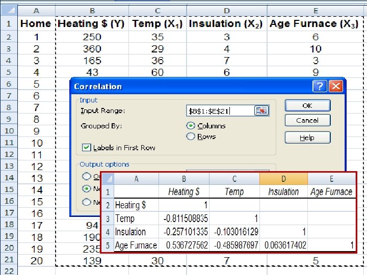
Multiple Linear Regression - Example Can we predict heating cost? Three variables are thought to relate to the heating costs: (1) the mean daily outside temperature, (2) the number of inches of insulation in the attic, and (3) the age in years of the furnace. To investigate, Salisbury's research department selected a random sample of 20 recently sold homes. It determined the cost to heat each home last January 14 -31

Multiple Linear Regression - Example
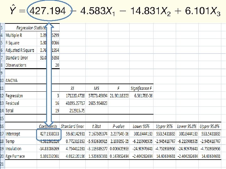
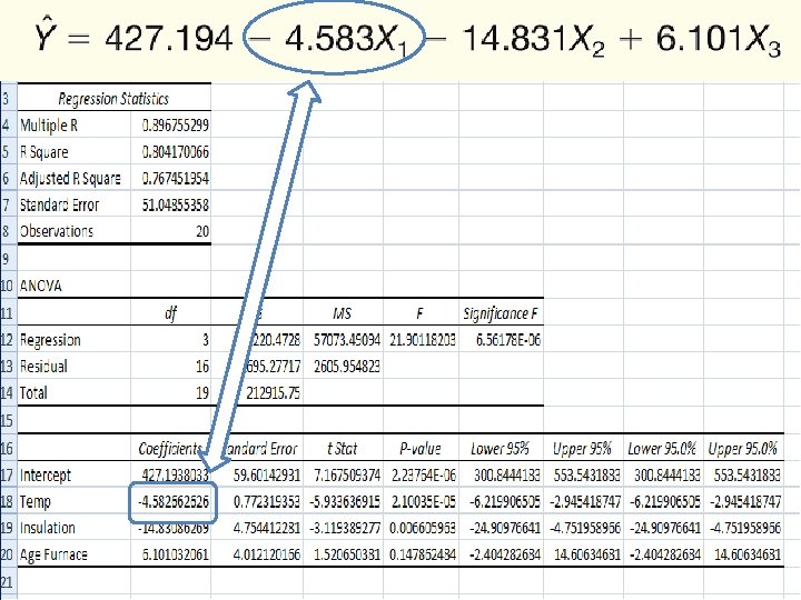
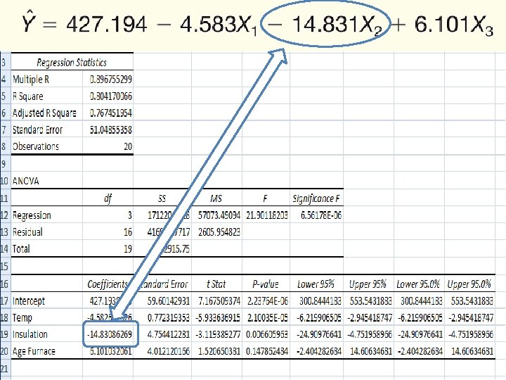

The Multiple Regression Equation – Interpreting the Regression Coefficients b 1 = The regression coefficient for mean outside temperature (X 1) is -4. 583. The coefficient is negative and shows a negative correlation between heating cost and temperature. As the outside temperature increases, the cost to heat the home decreases. The numeric value of the regression coefficient provides more information. If we increase temperature by 1 degree and hold the other two independent variables constant, we can estimate a decrease of $4. 583 in monthly heating cost.

The Multiple Regression Equation – Interpreting the Regression Coefficients b 2 = The regression coefficient for mean attic insulation (X 2) is -14. 831. The coefficient is negative and shows a negative correlation between heating cost and insulation. The more insulation in the attic, the less the cost to heat the home. So the negative sign for this coefficient is logical. For each additional inch of insulation, we expect the cost to heat the home to decline $14. 83 per month, regardless of the outside temperature or the age of the furnace.

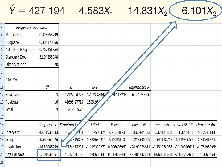
The Multiple Regression Equation – Interpreting the Regression Coefficients b 3 = The regression coefficient for mean attic insulation (X 3) is 6. 101 The coefficient is positive and shows a negative correlation between heating cost and insulation. As the age of the furnace goes up, the cost to heat the home increases. Specifically, for each additional year older the furnace is, we expect the cost to increase $6. 10 per month.

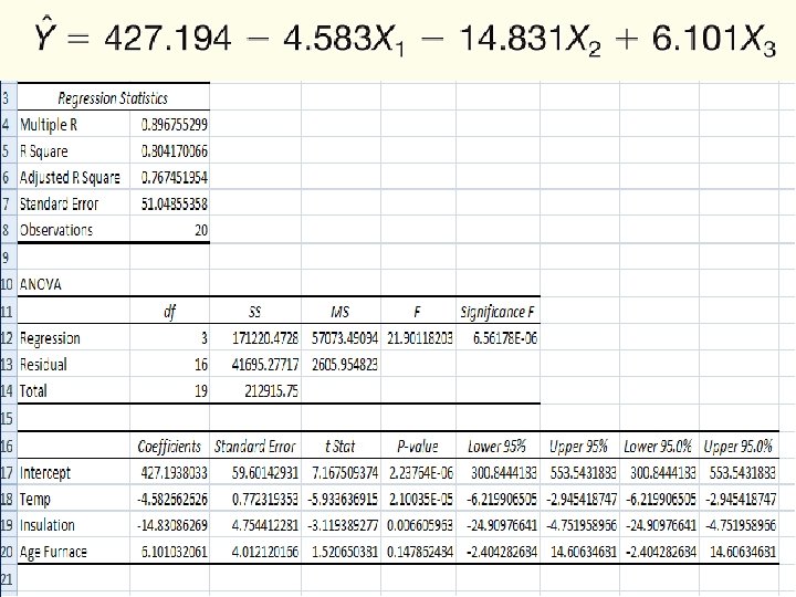
Applying the Model for Estimation What is the estimated heating cost for a home if: • the mean outside temperature is 30 degrees, • there are 5 inches of insulation in the attic, and • the furnace is 10 years old?

Multiple regression equations Very often we want to select students or employees who have the highest probability of success in our school or company. Andy is an administrator at a paralegal program and he wants to predict the Grade Point Average (GPA) for the incoming class. He thinks these independent variables will be helpful in predicting GPA. • High School GPA (X 1) • SAT - Verbal (X 2) • SAT - Mathematical (X 3) Andy completes a multiple regression analysis and comes up with this regression equation: Prediction line Y’ = b 1 X 1+ b 2 X 2+ b 3 X 3+ a Y’ = 1. 2 X 1+. 00163 X 2 -. 00194 X 3 -. 411 Y’ = 1. 2 gpa +. 00163 satverb -. 00194 satmath -. 411

Here comes Victoria, her scores are as follows: • High School GPA = 3. 81 • SATVerbal = 500 • SATMathematical = 600 Prediction line: Y’ = b 1 X 1+ b 2 X 2+ b 3 X 3+ a Y’ = 1. 2 X 1+. 00163 X 2 -. 00194 X 3 -. 411 What would we predict her GPA to be in the paralegal program? Y’ = 1. 2 gpa +. 00163 satverb -. 00194 satmath -. 411 Y’ = 1. 2 (3. 81) +. 00163 (500) -. 00194 (600) -. 411 Y’ = 4. 572 +. 815 - 1. 164 -. 411 = 3. 812 Predict Victor’s GPA, his scores are as follows: We predict Victoria will have a GPA of 3. 812 We predict • High School GPA = 2. 63 Victor will have a • SAT - Verbal = 469 GPA of 2. 656 • SAT - Mathematical = 440 Y’ = 1. 2 gpa +. 00163 satverb -. 00194 satmath -. 411 Y’ = 1. 2 (2. 63) +. 00163 (469) -. 00194 (440) -. 411 Y’ = 3. 156 +. 76447 -. 8536 -. 411 = 2. 66

Just for fun What if we were looking to see if our stop-smoking program affects peoples‘ desire to smoke. What would null hypothesis be? a. Can’t know without knowing the dependent variable b. The program does not work c. The programs works d. Comparing the null and alternative hypothesis Correct

Just for fun Correct Which of the following is a Type I error: a. We conclude that the program works when it fact it doesn’t b. We conclude that the program works when in fact it does c. We conclude that the program doesn’t work when in fact it does d. We conclude that the program doesn’t work when in fact it doesn’t

Just for fun What is the null hypothesis of a correlation coefficient? a. It is zero (nothing going on) b. It is less than zero c. It is more than zero d. It equals the computed sample correlation Correct

Just for fun In the regression equation, what does the letter "a" represent? a. Y intercept b. Slope of the line c. Any value of the independent variable that is selected d. None of these Correct Y’ = a + bx 1 + bx 2 + bx 3 + bx 4

Just for fun Assume the least squares equation is Y’ = 10 + 20 X. What does the value of 10 in the equation indicate? a. Y intercept b. For each unit increased in Y, X increases by 10 c. For each unit increased in X, Y increases by 10 d. None of these Correct

Just for fun In the least squares equation, Y’ = 10 + 20 X the value of 20 indicates a. the Y intercept. b for each unit increase in X, Y increases by 20. c. for each unit increase in Y, X increases by 20. d. none of these. Correct

Just for fun In the equation Y’ = a + b. X, what is Y’ ? a. Slope of the line b. Y intercept c. Predicted value of Y, given a specific X value d. Value of Y when X = 0 Correct

Just for fun If there are four independent variables in a multiple regression equation, there also four a. Y-intercepts (a). b. regression coefficients (slopes or bs). c. dependent variables. d. constant terms (k). Correct Y’ = a + bx 1 + bx 2 + bx 3 + bx 4
 is 0. 80, what")
Just for fun If the coefficient of determination (r 2) is 0. 80, what percent of variation is explained? a. 20% b. 90% c. 64% d. 80% Correct What percent of variation is not explained? a. 20% b. 90% c. 64% d. 80% Correct

Just for fun Which of the following represents a significant finding: a. p < 0. 05 b. t(3) = 0. 23; n. s. c. the observed t statistic is nearly zero d. we do not reject the null hypothesis Correct

Just for fun In multiple regression what is the range of values for a coefficient of regression? a. 0 to +1. 0 b. 0 to -1. 0 c. -1. 0 to +1. 0 d. -∞ to +∞ Correct Y’ = a + b 1 X 1 + b 2 X 2 + b 3 X 3

Just for fun Correct If r = 1. 00, which inference cannot be made? a. The dependent variable can be perfectly predicted by the independent variable b. This provides evidence that the dependent variable is caused by the independent variable c. All of the variation in the dependent variable can be accounted for by the independent variable d. Coefficient of determination is 100%.

Just for fun Winnie found an observed correlation coefficient of 0, what should she conclude? a. Reject the null hypothesis b. Do not reject the null hypothesis c. Not enough info is given Correct

Just for fun In a regression analysis what do we call the variable used to predict the value of another variable? a. Independent b. Dependent c. Correlation d. Determination Correct

Just for fun What can we conclude if the coefficient of determination is 0. 94? a. r 2 = 0. 94 b. direction of relationship is positive c. 94% of total variation of one variable is explained by variation in the other variable. d. Both A and C e. All of the above are correct Correct

Just for fun What is the range of values for a coefficient of determination? a. 0 to +1. 0 b. 0 to -1. 0 c. -1. 0 to +1. 0 d. -∞ to +∞ Correct

Just for fun Which of the following statements regarding the coefficient of correlation is true? a. It ranges from -1. 0 to +1. 0 b. It measures the strength of the relationship between two variables c. A value of 0. 00 indicates two variables are not related d. All of these Correct

Just for fun What does a coefficient of correlation of 0. 70 infer? (r = +0. 70) a. Almost no correlation because 0. 70 is close to 1. 0 b. 70% of the variation in one variable is explained by the other c. Coefficient of determination is 0. 49 d. Coefficient of nondetermination is 0. 30 Correct

Just for fun The Pearson product-moment correlation coefficient, r, requires that variables are measured with: a. an interval scale b. a ratio scale c. an ordinal scale d. a nominal scale e. either A or B. Correct

Just for fun If r = 0. 65, what does the coefficient of determination equal? a. 0. 194 b. 0. 423 c. 0. 577 d. 0. 806 Correct

Just for fun What is the measure that indicates how precise a prediction of Y is based on X or, conversely, how inaccurate the prediction might be? a. Regression equation b. Slope of the line c. Standard error of estimate d. Least squares principle Correct

Just for fun Agnes compared the heights of the women’s gymnastics team and the scores they got. If she doubled the number of players measured, but ended up with the same correlation (r) what effect would that have on the results? a. the r is the same, so the conclusion would be the same b. the r is the same, but with more people, degrees of freedom (df) would go up and it would be harder to reject the null hypothesis. c. the r is the same, but with more people, degrees of freedom (df) would go up and it would be easier to reject the null hypothesis. Correct

Just for fun Which of the following is true about the standard error of estimate? a. It is a measure of the accuracy of the prediction b. It is based on squared vertical deviations between Y and Y’ c. It cannot be negative d. All of these Correct Standard error of the estimate: • a measure of the average amount of predictive error • the average amount that Y’ scores differ from Y scores • a mean of the lengths of the green lines

Just for fun If all the plots on a scatter diagram lie on a straight line, (perfect correlation) what is the standard error of estimate? a. - 1 b. +1 c. 0 d. Infinity Correct Standard error of the estimate: • a measure of the average amount of predictive error • the average amount that Y’ scores differ from Y scores • a mean of the lengths of the green lines

Just for fun Scatterplot A Scatterplot B Scatterplot C Which of these correlations would be most likely to have the highest positive value for r? a. Scatterplot A b. Scatterplot B c. Scatterplot C d. Can not be determined from the information given Correct

Just for fun Scatterplot A Scatterplot B Scatterplot C Which of these scatterplots will have the smallest “y intercept”? a. Scatterplot A b. Scatterplot B c. Scatterplot C d. Can not be determined from the information given Correct

Just for fun Scatterplot A Scatterplot B Scatterplot C Which of these correlations would be most likely to represent the correlation between salary and expenses? a. Scatterplot A b. Scatterplot B c. Scatterplot C d. Can not be determined from the information given Correct

Just for fun Which of the following correlations would allow you the most accurate predictions? a. r = + 0. 01 b. r = - 0. 10 c. r = + 0. 40 d. r = - 0. 65 Correct

Just for fun After duplicate correlations have been discarded and trivial correlations have been ignored, there remain a. two correlations b. three correlations c. six correlations d. nine correlations Correct

Just for fun Which of the following conclusions can not be made from the data in the matrix? a. There is a significant correlation between Science and Reading b. There is a significant correlation between Math and Reading c. There is a significant correlation between Math and Science Correct

- Slides: 75